Model based testing with graph grammers

(1)

Model-Based Testing with

Graph Grammars

MSc Thesis (Afstudeerscriptie)

written by

Vincent de Bruijn

Formal Methods & Tools,

University of Twente,

Enschede,

The Netherlands

[email protected]

(2)

Abstract

Graph Grammars describe system behavior through graphs and graph transformation rules. Graph Grammars have not been used for Model-Based Testing. However, Graph Grammars have many structural advantages, which are potential benets for the model-based testing process. We de-scribe a model-based testing setup with Graph Grammars. The result is a system for automatic test generation from Graph Grammars. A graph transformation tool, GROOVE (GRaphs for Object-Oriented VErication), and a model-based testing tool using Symbolic Transition Sys-tems, ATM (Axini TestManager), are used as the backbone of the system.

(3)

ACKNOWLEDGEMENTS

First I would like to thank my supervisors: Arend Rensink, Marielle Stoelinga, Axel Belinfante and Machiel van der Bijl. All the energy and time put into giving me feedback, helping me when I got stuck and pushing me to do better has been greatly appreciated.

I would like to thank my current employers at Axini B.V. for providing the opportunity to do this master thesis and for giving me ample time to nish it.

I would like to also thank my fellow nal year students: Freark van den Berg, Harold Bruintjes, Ronald Burgman, Paul Stapersma, Gerjan Stokkink and Lesley Wevers. Even though we were not always productive, the discussions while drinking coee or beer have been fun.

(4)

Introduction

In this introduction, rst the importance of testing and automation of testing is stressed. Then Model-Based Testing is shown to be a useful tool for automation of testing. Graph Grammars and graph transformation are argued to be useful as formalism for Model-Based Testing. Some leading tools for automatic test generation are set out, which include the tools used in this report. The research goals are given and nally a roadmap explains the basic structure of the rest of this report.

1.1 Testing

In software development projects, often time and budget costs are exceeded. Laird and Bren-nan [13] investigated in 2006 that 23% of all software projects are canceled before completion. Furthermore, of the completed projects, only 28% are delivered on time with the average project overrunning the budget with 45%. The cause of this often are the unclear ambigious requirements of the software system to develop.

Testing is an important part of software development, because it decreases future maintainance costs [19]. Testing is a complex process and should be done often [22]. Therefore, the testing process should be as ecient as possible in order to save resources.

Test automation allows repeated testing during the development process. The advantage of this is that bugs are found early and can therefore be xed early. A widely used practice is maintaining a test suite, which is a collection of test-cases. However, when the creation of a test suite is done manually, this still leaves room for human error [16]. The process of deriving tests tends to be unstructured, barely motivated in the details, not reproducible, not documented, and bound to the ingenuity of single engineers [31].

1.2 Model-based Testing

(7)

A model can be used to systematically generate tests for the system. This is referred to as Model-Based Testing. Generating tests automatically leads to a larger test suite than if done manually. A large, systematically built test suite is bound to nd more bugs than a smaller, manually built one.

Models are created from the specication documents provided by the end-user. These specication documents are `notoriously error-prone' [18]. This implies that the model itself needs validation. Validating the model usually means that the requirements themselves are scrutinised for consis-tency and completeness [31]. This helps to clear up ambigious requirements early on, which allows better estimation of the budget and time demands.

The stakeholders evaluate the constructed model to verify its correctness. However, the visual or textual representation of large models may become troublesome to understand, which is re-ferred to as the model having a low model transparency or high model complexity. The problem with transition systems is that a larger number of states and/or transitions decreases the model transparency. We think that low model transparency make errors harder to detect and that it ob-structs the feedback process of the stakeholders. Using models with high transparency is therefore essential.

1.3 Graph Transformation

A formalism that claims to have higher model transparency is Graph Transformation. The system states are represented by graphs and the transitions between the states are accomplished by applying graph change rules to those graphs. These rules can be expressed as graphs themselves. A graph transformation model of a software system is therefore a collection of graphs, each a visual representation of one aspect of the system. This formalism may therefore provide a more intuitive approach to system modelling than traditional state machines. Graph Transformation and its potential benets have been studied since the early '70s [23]. The usage of this computational paradigm is best described by the following quote from Andries et al. [1]:

Graphs are well-known, well-understood, and frequently used means to represent sys-tem states, complex objects, diagrams, and networks, like owcharts, entity-relationship diagrams, Petri nets, and many more. Rules have proved to be extremely useful for de-scribing computations by local transformations: Arithmetic, syntactic, and deduction rules are well-known examples.

An informative paper on graph transformations is written by Heckel et al. [10]. A quote from this paper:

Graphs and diagrams provide a simple and powerful approach to a variety of problems that are typical to computer science in general, and software engineering in particular.

1.4 Tools

Tools for model-based testing and tools for graph transformation already exist. The leading tools in these areas are investigated in this section.

The testing tool developed by Axini1_{is used for the automatic test generation on symbolic models,}

which combine a state and data type oriented approach. This tool is referred to as Axini Test Manager (ATM) and is used in practice by several Dutch companies.

(8)

• TorX [28]: accepts behaviour models such as I/O labelled transition systems. A version of

this tool written in Java under continuous development is JTorX [2]. This version accepts the same kind of models as ATM.

• Spec Explorer[32]: provides a model editing, composition, exploration and visualization

environment within Visual Studio, and can generate oine .NET test suites or execute tests as they are generated (online).

• JUMBL[24]: an academic model-based statistical testing that supports the development of

statistical usage-based models using Markov chains, the analysis of models, and the genera-tion of test cases.

• AETG[5]: implements combinatorial testing, where the number of possible combinations of

input variables are reduced to a few `representative' ones.

• STG tool[4]: implements conformance testing techniques to automatically derive symbolic

test cases from formal operational specications.

Table 1.1 shows the graph transformation tools that participated at the Transformation Tool Contest 2011 in Zurich[7]. A comparison based on their strong points is shown taken from [12].

1.5 Research goals

The motivation above is given for using graph grammars as a modelling technique in Model-Based Testing. The goal of this research is to create a system for automatic test generation on graph grammars. If the assumptions that graph grammars provide a more intuitive modelling and testing process hold, this new testing approach will lead to a more ecient testing process and fewer incorrect models. The system to be designed, once implemented and validated, should provide a valuable contribution to the testing paradigm.

The backbone of this system consists of two tools: a model-based testing tool for the testing part and a graph transformation tool for visual editing and state-space exploration of Graph Grammars. The choice was made to use ATM as the model-based testing tool, because of the location of Axini, their willingness to support this project and the already available models for case studies. Another interesting option for our research would have been to use an open-source MBT tool. In particular JTorX was an interesting candidate due to its maturity and the available support at the University of Twente. The tools GROOVE and ATM are used to create this system. The graph transformation tool GROOVE2 _{does state-space exploration, has a visual editor and}

has available support at the University of Twente, therefore it is used to model and explore the graph grammars.

The research goals are split into a design and validation component:

1. Design: Design and implement a system using ATM and GROOVE which performs Model-Based Testing on graph grammars.

2. Validation: Validate the design and implementation using case studies and performance measurements.

The result of the design goal is one system called the GROOVE-Axini Testing System (GRATiS). The validation goal uses case-studies with existing specications from systems tested by Axini. Each case-study has a graph grammar and a symbolic model which describe the same system. GRATiS and ATM are used for the automatic test generation on these models respectively. Both the models and the test processes are compared as part of the validation.

(9)

Suitability and strong points of the tool

ATL/EMFTVM: general-purpose model transformation.

ATL is a mature language for mapping input models to output models. The EMFTVM runtime introduces composition and rewriting.

Edapt: model migration in response to metamodel adaptation. High automation by reuse of recurring migration specications. In-place transformation, seamless metamodel editor integration. GrGen.NET: general-purpose graph rewriting.

Pattern matching of high performance and expressiveness; highly programmable. Excellent debugging and documentation. Focus on compilers, computer linguistics. GROOVE: state space exploration, general-purpose graph rewriting.

Rapid prototyping, visual debugging, model checking.

Expressive language (nested rules, transactions, control); isomorphism reduction. Henshin: graph transformations for EMF models with explicit control ow. Expressive language (nested rules, support for higher-order transformations) JavaScript support, light-weight model & API, state space analysis

MDELab SDI: graph transformations for EMF models with explicit control ow. Expressive language, mature graphical editor, support for debugging at model level. High exibility, easy integration with other EMF/Java applications.

metatools: general-purpose model transformations.

Seamless integration of hand-written and generated sources, of imperative and declarative style. Full access to host language, libraries and legacy code. MOLA: general-purpose model transformations with explicit control ow.

Expressive language, graphical editor with graphical code completion and refactorings, built-in metamodel editor, EMF support.

QVTR-XSLT: general-purpose model transformations.

Supporting the graphical notation of QVT Relations with a graphical editor to dene transformations, and generate executable XSLT programs for them. UML-RSDS: general-purpose model transformation with verication support. Declarative transformation specication using only UML/OCL.

Ecient compiled transformation implementations.

Viatra2: general-purpose multi-domain model transformations. Model space with arbitrary metalevels, excellent programming API. Incremental pattern matching.

Table 1.1: Graph transformation tools and their strong points

1. A graph grammar must be used as the model; it must derive from the specication and be used for the testing.

2. It must be possible to measure the test progress/completion, by means of coverage statistics (explained in detail in section 2.1.2).

3. The solution must be ecient: it should be usable in practice, therefore the technique should be scalable and the imposed constraints reasonable from a practical view point.

The implementation described in chapter 4 upholds all three requirements; this is elaborated in chapter 6.

1.6 Roadmap

(10)

(11)

Chapter 2

Background

The structure of this chapter is as follows: the general model-based testing process is set out in section 2.1. Some basic concepts from algebra are described in section 2.2. Then the symbolic models used by ATM are described in section 2.3. Section 2.4 describes the Graph Grammar formalism. GROOVE and ATM are described in section 2.5.

2.1 Model-based Testing

Model-based testing is a testing technique where a System Under Test (SUT) is tested for con-formance to a model description of the system. The general setup for this process is depicted as a UML sequence diagram in Figure 2.1. The specication of a system is provided as a model to a test derivation component which generates a test suite. The test suite is used by a test execution component to test the SUT. Tests are executed by providing input/stimuli to the SUT and monitoring the output/response. The test execution component evaluates whether the correct responses are given. It gives a 'pass' or 'fail' verdict depending on whether the SUT conforms to the model or not.

Test Derivation

Test

Execution SUT

Verdict Pass/Fail

Speciﬁcation

stimuli

response

Figure 2.1: A general model-based testing setup

This type of based testing is called batch testing or oine testing. Another type of model-based testing is on-the-y testing. The main dierence is that no test cases are derived, instead a transition in the model is chosen and tested on the system directly. The general architecture for this process is shown in Figure 2.2. An example of an on-the-y testing tool is TorX [28]. Variations of state machines and transition systems have been widely used as the underlying model for test generation. Other tools use the structure of data types to generate test data.

(12)

Test Engine

SUT

Verdict Pass/Fail

Speciﬁcation input output

stimulus response

Figure 2.2: A general 'on-the-y' model-based testing setup

understand the models in the rest of the paper, namely Graph Grammars and Symbolic Transition Systems. Next, an adaptation of Labelled Transition Systems, the Input-Output Transition System is described. This is a useful formalism for Model-Based Testing. Finally, the notion of coverage is explained.

2.1.1 Previous work

Transition-based formal testing theory was introduced by De Nicola et al. [21]. The input-output behavior of processes is investigated by series of tests. Two processes are considered equivalent if they pass exactly the same set of tests. This testing theory was rst used in algorithms for automatic test generation by Brinksma [3]. This led to the so-called canonical tester theory. Tretmans gives a formal approach to protocol conformance testing (whether a protocol conforms to its specications) in [29] and an algorithm for deriving a sound and exhaustive test suite from a specication in [30]. A good overview of model-based testing theory and past research is given in "Model-Based Testing of Reactive Systems" [17].

2.1.2 Labelled Transition Systems

A Labelled Transition System (LTS) is a structure consisting of states with labelled transitions between them.

Denition 2.1.1. Labelled Transition Systems An LTS is a 4-tuplehQ, L, T, q0i, where:

• Qis a nite, non-empty set of states • L is a nite set of labels

• T ⊆Q×(L∪ {τ})×Q, withτ /∈L, is the transition relation • q0∈Qis the initial state.

We writeq−→µ q0 if there is a transition labelledµfrom stateqto stateq0, i.e.,(q, µ, q0)∈T. q, q0

are called the source and target states of the transition respectively. The informal idea of such a transition is that when the transition system is in stateqit may perform actionµ, and go to state q0.

(13)

IOTSs have the same denition as LTSs with one addition: each label l ∈ L has a type ι ∈Y,

where Y = {input, output}. Each label can therefore specify whether the action represented by

the label is a possible input or an expected output of the system under test. An IOTS is formally dened as:

Denition 2.1.2. Input-Output Transition Systems

An IOTS is a 4-tuplehQ, L, TY, q0i, whereTY ⊆T×Y are the input-output transitions.

When the transition system is in the source state of an input transition, the input can be given to the SUT. When the transition system is in the source state of an output transition, the output should be observed from the SUT. In both cases, the transition system advances to the target state of the transition. The case where a state has both input and output transitions is not considered in this report.

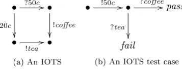
An example of such an IOTS is shown in Figure 2.3a. This system allows an input of 20 or 50 cents and then outputs tea or coee accordingly. The inputs are preceded by a `?', the outputs are preceded by an `!'. This system is a specication of a coee machine. A test case can also be described by an IOTS with special pass and fail states.

A test case for the coee machine is given in Figure 2.3b. The test case shows that when an input of `50c' is given, an output of `coee' is expected from the tested system, as this results in a `pass' verdict. When the system responds with `tea', the test case results in a `fail' verdict. The pass and fail verdicts are two special states in the test case, which are sink states, i.e., once in either of those the test case cannot leave that state.

Test cases should always reach a pass or fail state within nite time. This requirement ensures that the testing process halts.

• ?50c //

?20c

•

!coffee

•

!tea //• (a) An IOTS

• !50c //• ?coffee//

?tea

pass

fail

[image:13.595.211.390.442.510.2]

(b) An IOTS test case

Figure 2.3: The specication of a coee machine and a test case as an IOTS

Coverage The number of tests that can be generated from a model is potentially innite. There-fore, there must be a test selection strategy to maximize the quality of the tests while minimizing the time spent testing. Coverage statistics help with test selection. Coverage statistics are calcu-lated to indicate how adequately the testing has been performed [33]. These statisics are therefore useful metrics for communicating how much of a system is tested.

One type of coverage is white-box coverage or code coverage: This coverage statistic measures how much of the lines of codes in the implementation is tested. A line of code is considered tested when it is executed during the test run.

(14)

1. the transition is a stimulus and the input represented by the label of the transition is given to the SUT

2. the transition is a response and the output represented by the label of the transition is observed from the SUT

State coverage can be measured by dividing the tested states by the total states in the model. The same process applies to transition coverage. As an example, the coverage metrics of the IOTS test case example in 2.3b are calculated. The test case tests one path through the specication and passes through 3 out of 4 states and 2 out of 4 transitions. The state coverage is therefore 75% and the transition coverage is 50%.

This example shows that the total number of states and transitions in the transition systems has to be known; coverage statistics cannot be measured on an innitely large LTS, for example.

2.2 Algebra

Some basic concepts from algebra are described here. For a general introduction into logic we refer to [11]. This section explains in order: multi-sorted signatures, algebrae, variables & terms and term-mapping & valuations. The algebra described here will be used in the next sections to formally dene Symbolic Transition Systems and Graph Grammars.

Denition 2.2.1. Multi-sorted Signatures

A multi-sorted signature hS, Fi describes the sorts and function symbols of a formal language. S is a set of sorts. F is a set of function symbols. Each f ∈ F has an arity n ∈ N, where

a function symbol with arity n = 0 is called a constant symbol. Fi denotes the subset of F

with function symbols of arity n = i. The sort of a function symbol f ∈ F with arity n is

given by σ(f) = s1...sn+1, withsi ∈ S for1 ≤ i ≤n. sn+1 is the return sort. In this report,

S = {int,real,bool,string} denoting the integer, real, boolean and string sorts respectively. F

features the commonly used function symbols, which include, but are not restricted to, `int:+', `string:=', `¬', `1', which are the addition of integers, the equality of strings, the negation of a

boolean and the integer `one' respectively. The sorts and arities of these examples are given by: 1. σ(int :+) =hint, int, inti

2. σ(string : =) =hstring, string, booli

3. σ(¬) =hbool, booli

4. σ(1) =hinti

Denition 2.2.2. Algebrae

An algebra A=hU,Φihas a non-empty set Uof values called a universe, partitioned intoUs for

eachs∈S, and a setΦof functions. A functionφAis typedUsA1×...U

sn

A →U

sn+1

A , wheres1...sn+1

is the sort of the function symbol given by the signature. For example,<A:UintA ×UintA →UboolA

represents the `less-than' comparison of two integers.

Denition 2.2.3. Point algebra

We dene a point algebra P to be an algebra with∀s∈S.|UsP|= 1.

Denition 2.2.4. Variables

We dene V =Vint_{] V}real_{] V}bool_{] V}string _{to be the set of variables. Terms over} _V_{, denoted}

T(V), are built from function symbolsF and variablesV ⊆ V. The denition of a term is: t ::= f(t1...tn) , wherenis the arity of φ

(15)

We writevar(t)to denote the set of variables appearing in a termt∈ T(V). Terms t∈ T(∅)are

called ground terms. An example of a termt is(x+ (y−1)), withvar(t) ={x, y}. The type of a

term is given by:

σ:t7→ s if t=x∈ Vs

sn+1 if t=f(t1...tn)andσ(f) =s1...sn+1, providedσ(ti) =si

The set of terms with return type bool, is denoted as B(V). An example is(x < y), where the

result istrue orfalse.

Denition 2.2.5. Term-mapping

A term-mapping is a functionµ:V → T(V). A valuation ν is a function ν :V →Uthat assigns

values to variables. For example, given an algebra,ν :{(x7→1),(y7→2)}assigns the values 1 and

2 to the variablesxandy respectively. A valuation of a term givenAis dened by:

ν : x 7→ ν(x)

f(t1...tn) 7→ fA(ν(t1)...ν(tn))

When every variable in a term is dened by a valuation, the term can be valuated to a value. Therefore, when every variable in a term-mapping is dened by a valuation, a new valuation can be obtained. Formally, this is dened as: _af ter_: (V →_U)×(V → T(V))→(V →_U). Given

a valuationν and a term-mappingµ, (νafterµ) :ν7→ν(µ(ν)).

2.3 Symbolic Transition Systems

Symbolic Transition Systems (STSs) combine a state oriented and data type oriented approach. This formalism is a specication of system behavior like LTSs. These systems are used in practice in ATM and will therefore be part of GRATiS. In this section, previous work on STSs is reviewed. The denitions of STSs and IOSTSs follow. An example of an IOSTS is then given. Next, the mapping of an STS to an LTS is explained and illustrated by an example. This mapping is useful when comparing STSs to Graph Grammars, because both systems can be mapped to an LTS and then compared. Finally, dierent coverage metrics on STSs and the relation with LTS coverage metrics are explained.

2.3.1 Previous work

STSs are introduced by Frantzen et al. [14]. This paper includes a detailed denition, on which the denition below is based. The authors also give a sound and complete test derivation algorithm from specications expressed as STSs. Deriving tests from a symbolic specication, also called Symbolic test generation, is introduced by Rusu et al. [27]. Here, the authors use Input-Output Symbolic Transition Systems (IOSTSs). These systems are very similar to the STSs in [14]. However, the denition of IOSTSs we will use in this report is based on the STSs by [14]. A tool that generates tests based on symbolic specications is the STG tool, described in Clarke et al. [4].

2.3.2 Denition

An STS has locations and switch relations. If the STS represents a model of a software system, a location in the STS represents a state of the system, not including data values. A switch relation denes the transition from one location to another. The location variables are a representation of the data values in the system. A switch relation has a gate, which is a label representating the execution steps of the system. Gates have interaction variables, which represent some input or output data value. Switch relations also have guards and update mappings. A guard is a term

(16)

false. When the valuation results in true, the switch relation of the guard is enabled. An update mapping is a term-mapping of location variables. After the system switches to a new location, the variables in the update mapping will have the value corresponding to the valuation of the term.

Denition 2.3.1. Symbolic Transition Systems

A Symbolic Transition System is a tuplehW, w0,L, ı,I,Λ, Di, where:

• W is a nite set of locations. • w0∈W is the initial location.

• L ⊆ V is a nite set of location variables.

• ıis a term-mappingL → T(∅), representing the initialisation of the location variables. • I ⊆ V is a set of interaction variables, disjoint fromL.

• Λis a nite set of gates. The unobservable gate is denotedτ(τ /∈Λ); we writeΛτ forΛ∪ {τ}.

The arity of a gateλ∈Λτ, denotedarity(λ), is a natural number. The parameters of a gate

λ∈Λτ, denoted param(λ), are a tuple of length arity(λ)of distinct interaction variables.

We x arity(τ) = 0, i.e. the unobservable gate has no interaction variables.

• D⊆W×Λτ× B(L ∪ I)×(L → T(L ∪ I))×W, is the switch relation. We writew λ,γ,ρ

−−−→w0

instead of (w, λ, γ, ρ, w0) ∈ D, where γ is referred to as the guard and ρ as the update

mapping. We require(var(γ)∪var(ρ))⊆(L ∪param(λ)). We deneout(w)⊆Dto be the

outgoing switch relations from location w.

An IOSTS can now easily be dened. The same dierence between the labels in LTSs and IOTSs apply, namely each gate has a typeι∈Y. As with labels, each gate is preceded by an `?' or `!'

to indicate whether it is an input or an output respectively. The full denition is as follows:

Denition 2.3.2. Input-Output Symbolic Transition Systems

An IOSTS is a 5-tuplehW,L, ı,ΛY, Di, whereΛY ⊆Λ×Y are the input-output gates.

2.3.3 Example

In Figure 2.4 the IOSTS of a simple board game is shown, where two players consecutively throw a die and move along four squares, which are situated in a circle. The switch relation without source location is a graphical representation of the variable initializationı. The values in the tuple

of the IOSTS are dened as follows:

W = {t, m}

w0 = t

L = {T, P1, P2, D}

ı = {T 7→0, P17→0, P27→2, D7→0} I = {d, p, l}

Λ = {?throw,!move}

D = {t−−−−−−−−−−−−−→?throw,1≤d≤6,D7→d m,

m−−−−−−−−−−−−−−−−−−−−−−−−→!move,T=1∧l=(P1+D)%4,P17→l,T7→2 t, m−−−−−−−−−−−−−−−−−−−−−−−−→!move,T=2∧l=(P2+D)%4,P27→l,T7→1 t}

The variablesT, P1, P2 and D are the location variables symbolizing the player's turn, the

po-sitions of the players and the number of the die thrown respectively. The output gate !move

has param= hp, lisymbolizing which player moves to which location. The input gate ?throws

hasparam =hdisymbolizing which number is thrown by the die. The switch relation with gate

(17)

update sets the location variable D to the value of interaction variabled. The switch relations

with gate!move have the restriction that it must be the turn of the player moving and that the

new location of the player is the number of steps ahead as thrown by the die. The update mapping sets the location of the player to the correct value and passes the turn to the next player. Figure 2.4 shows the example visually. The gates, guards and updates are separated by pipe symbols `|' respectively. The initialization function is expressed by a switch relation with no source location, gate and guard.

T7→1, P17→0, P27→2, D7→0 _/_/

t ?throws(d:N)|1<=d <= 6|D7→d //m

!move(p:N,l:N)|T=1∧p=1∧l=(P1+D)%4|P17→l, T7→2

u

!move(p:N,l:N)|T=2∧p=2∧l=(P2+D) %4|P27→l, T7→1

i

Figure 2.4: The IOSTS of a board game example

2.3.4 STS to LTS mapping

This section shows the method of mapping an STS to an LTS.

Consider an STS J. We can construct an LTS K from J, such that K is an expansion of J.

There exists a mapping from the location and location variable valuations to the states ofKand

from the switch relations and variable valuations ofJ to the transitions ofK. These relations are

dened as follows:

Denition 2.3.3. STS-to-LTS mapping

µQ : (W×(L →U))→Q

µL : (Λ×(I →U))→L

µT : (w λ,γ,ρ

−−−→w0, ν: ((L ∪ I)→_U))7→(µQ(w, νL)

µL(λ,νI)

−−−−−−→µQ(w0,(νafter ρ)L))

When the number of possible valuations forLandI is nite, the transformation is always possible

to an LTS with nite number of states. This often is the case when the guards of the switch relations provide bounds to the interaction variables and the update mappings do not inntely increase of decrease the location variables.

An example of this transformation is shown in Figure 2.5. The label `do(1)' in the LTS is a textual representation of the gate `do' plus a valuation of the interaction variable `d'. The text on the nodes indicate from which location and valuation the state was created. The node labelled `w0, N= 2' is an example of an unreachable state.

2.3.5 Coverage

(18)

init|true|N:= 0;

•

do(d:N)|1<=n <= 2|N:=n

•

sub(i:N)|1<=i <= 2|N:=N−i

G

(a) The STS

w0, N= 2 // w0, N= 0

do(1) w w do(2) ! !

w1, N= 1

sub(1) 7 7 sub(2) ! !

w0, N= 1

do(1)

o

o do(2) -- w1, N = 2

sub(1) m m sub(2) a a

w0, N=−1

do(1) a a do(2) : : t t t t t t t t t t t t t t t t t t t t

[image:18.595.160.439.114.397.2]

(b) The LTS

Figure 2.5: An example of a transformation of an STS to an LTS

2.4 Graph Grammars

A Graph Grammar (GG) is also a specication of system behavior like LTSs and STSs are. A GG is composed of a set of graph transformation rules. These rules indicate how a graph can be transformed to a new graph. These graphs are called host graphs. The rules are composed of graphs themselves, which are called rule graphs.

The rest of this section is ordered as follows: rst, graphs, host graphs, rule graphs and graph transformation rules are explained. Then, the denition of a Graph Transition System (GTS) is given. An example of a GG and a GTS is then given. Finally, the denition of IOGGs is given. For a more detailed overview of GGs, we refer to [25, 10, 1].

Denition 2.4.1. Graphs

A graph is composed of nodes and edges. In this report, we assume a universe of nodes V = W]U] V ]2T, where W is the universe of standard graph nodes. The other symbols were

introduced in section 2.2; these are the universe of values, the universe of variables and the power set of the universe of terms respectively. E⊆V×L×Vis the universe of edges.

Denition 2.4.2. Host graphs

A host graphGis a tuplehVG, EGi, where:

• VG⊆(W]U)is the node set ofG

• EG ⊆(VG\U×L×VG)is the edge set of G

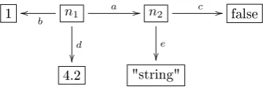
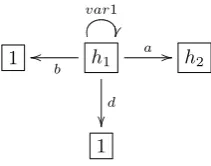
Figure 2.6 shows an example of a host graph. Here,n1, n2 ∈W are the identities of the nodes.

(19)

1 n1

b

o

d

a _/_/

n2 c //

e

false

[image:19.595.207.396.109.173.2]

4.2 "string"

Figure 2.6: An example of a host graph

Denition 2.4.3. Rule graphs

A rule graphH is a tuplehVH, EHi, where:

• VH ⊆(V\U)is the node set ofH

• EH ⊆(VH×L×VH)is the edge set ofH

In addition, the following must hold:

• ∀z∈VH∩2T .var(z)⊆VH - The variables used in the terms must be present as nodes in

the rule graph.

• ∀z∈VH∩z ∈ V.∃(_,_, z)∈EH - If a variable is used in a rule graph, it needs context.

Therefore, there must be an edge with the variable node as target.

Figure 2.7 shows an example of a rule graph. Here,r1, r2∈Ware the node identities,x1, x2∈ Vint

and {x1+ 1, x2} ∈2T. The set of terms is mapped as a node to the same value. This mapping

is explained in the next denition. The consequence is that this node implicitly expresses the relationx1+ 1 =x2.

int:x1 r1

b

o

d

a // _r

2 x1+ 1, x2

int:x2

Figure 2.7: An example of a rule graph

Denition 2.4.4. Morphisms

A graphghas a morphism to a graphg0 if there is a structure-preserving mapping from the nodes

and the edges of g to the nodes and the edges of g0 respectively. Elements of this mapping are

called images ing0 _{and pre-images in}_g_{. A graph}_g _{has a partial morphism to a graph}_g0 _{if there}

are elements ing without an image in g0_{. For morphisms between host graphs and between rule}

graphs, the pre-image and image must be the same node. The next denition gives the rule for morphisms from rule graphs to host graphs.

Denition 2.4.5. Host graph images for rule graphs

A rule graphH to a host graphGmorphism is a structure-preserving mapping, such that: • A node z∈Whas an imageiin Gifi=z

• A valuex∈Uhas an imageiin Gifi=x

• A variable v ∈ Vs_{, s}_∈ _S _{has an image} _i _in _G_if _i _∈

Us. This gives a valuation ν for the

variables in the rule graphs to the value nodes in the host graph.

(20)

Denition 2.4.6. Transformation rules

A transformation ruleris a tuplehLHS,NAC,RHS, li, where: • LHS is a rule graph representing the left-hand side of the rule

• NAC is a set of rule graphs representing the negative application conditions

• RHS is a rule graph representing the right-hand side of the rule

• l∈L is the label of the rule

There exist implicit partial morphisms from theLHS to each rule graph in NAC and from the LHS to theRHS by means of the node identities. These morphisms are rule graph morphisms.

Denition 2.4.7. Creators and erasers

A creator is an edge or node in theRHS of a rule, that is not in theLHS of the rule. An eraser is an edge or node in theLHS of a rule that is not in theRHS of that rule.

Denition 2.4.8. Rule matches

A rule r has a rule match on a host graph Gif its LHS has a morphism to Gand none of the

graphs inNAC have a morphism extending the morphism of theLHS toG. The morphism of the

LHS to a host graph is a match morphism m∈M.

Denition 2.4.9. Rule transitions

Letrbe a rule,Ga host graph andm a match morphism. Aftermis found, all nodes and edges

inLHS that do not have an image inRHS, are removed fromG. All elements inRHS that do not have a pre-image in LHS, are added toG. The result of this process is called a rule transition,

denoted by: G−−→r,m G0.

Figure 2.8 shows an example of the initial graphG0, one rule of a GG and the corresponding rule

match. G0 can be represented by h{n1, n2},{hn1, a, n1i,hn1, A, n2i,hn2, B, n2i}i. TheLHS of

the rule has a match inG0. NeitherNAC1 andNAC2 have a match inG0, because the edge with

label C does not exist inG0. The new graph after applying the rule isG1. The edge with label

ais removed from the graph and an edge with label bis added with the same source and target

node as the removed edge.

LHS r1

A

Z

Z a //r2

B Z Z NAC1 r1 A Z

Z a //r2

C Z Z NAC2 r1 A Z

Z b //r2

C

Z

G0

n1 b //n2

A

Z

Z a //n3

B Z Z RHS r1 A Z

Z b //r2

B

Z

G1

n1 b //n2

A

Z

Z b //n3

B

Z

rule graph morphism rule graph morphism

rule graph morphism

partial morphism

match morphism partial morphism

Figure 2.8: An example of a graph transformation

Denition 2.4.10. Graph Grammars A graph grammar is a tuplehR, G0i, where:

(21)

• G0 is the initial graph

By repeatedly applying graph transformation rules to the start graph and all its consecutive graphs, a GG can be explored to reveal a Graph Transition System (GTS). This transition system consists of graphs connected by rule transitions.

Denition 2.4.11. Graph Transition Systems

A graph transition system is a tuplehG, R, M, U, G0i, where:

• G is a set of graphs

• L⊆R×M is a set of labels

• U ⊆ G ×L× Gis the rule transition relation • G0∈ G is the initial graph

LetK =hR, G0i. A GTSO =hG, R, M, U, G0iis derived fromK by the following. G, M, U are

the smallest sets, such that:

• G0∈ G

• ifG∈ G andG−−→r,m G0 thenG0∈ G,(r, m)∈L,(G−−→r,m G0)∈U

In order to specify stimuli and responses with GGs, a denition is given for an Input-Output GG (IOGG).

Denition 2.4.12. Input-Output Graph Grammars

An IOGG is a tuplehRY, G0i, whereRY ⊆R×Y are input-output transformation rules.

Exploring an IOGG leads to an Input-Output Graph Transition System (IOGTS).

Denition 2.4.13. Input-Output Graph Transition Systems An IOGTS is a tuplehG, RY, M, UY, G0i, where:

• LY ⊆RY ×M are the input-output labels

• UY ⊆ G ×LY × Gare the input-output rule transitions

Denition 2.4.14. Rule priorities

A graph grammar with rule priorities P assigns a priorityp∈Nto ar∈R, such thatr7→p∈P.

The denition of GTSs is extended with this denition of rule priorities and the following:

r1, r2∈R, G∈ G.(G

r1,m1

−−−−→G0)∈U∧P(r1)> P(r2)→@m2, G00: (G

r2,m2

−−−−→G00)∈U

In the graph grammar in Figure 2.9, the `add' rule produces a rule transition to a graph, where thesubrule produces a rule transition back to the start graph. Suppose P(add)> P(sub), then

the `sub' rule does not have a outgoing rule transition from the start graph.

2.5 Tooling

2.5.1 ATM

(22)

A a // 1 (a) The initial graph

A a //

int: x x < 2 (b) TheLHSof theaddrule

A a //

x + 1 (c) The RHS of the addrule

A a // int: x x > 0 (d) TheLHSof thesubrule

[image:22.595.93.512.348.592.2]

A a // x - 1 (e) The RHS of the subrule

Figure 2.9: Priority rules

continuous development by Axini.

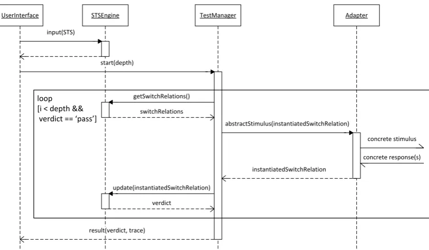
A UML sequence diagram for ATM is shown in Figure 2.10, depicting a test run from start to end.

UserInterface STSEngine TestManager Adapter

input(STS)

start(depth)

getSwitchRelations()

switchRelations

abstractStimulus(instantiatedSwitchRelation)

instantiatedSwitchRelation

concrete stimulus

concrete response(s) loop

[i < depth && verdict == ‘pass’]

update(instantiatedSwitchRelation)

verdict

result(verdict, trace)

Figure 2.10: ATM sequence diagram

The tool functions as follows:

1. An STS is given to an STS Engine, which keeps track of the current location and variables. The user starts the test and gives a `depth', indicating how many stimuli should be tested. The variablei stands for the current iteration ofloopand is initially set to 0. The variable verdictis initially set to0pass0.

(23)

a random strategy or a strategy using boundary-value analysis. The choice is represented by an instantiated switch relation.

3. The instantiated switch relation is given to the Test Execution component as an abstract stimulus. The term abstract indicates that the instantiated switch relation is an abstract representation of some computation steps taken in the SUT. For instance, a transition with label `?connect' is an abstract stimulus of the actual setup of a TCP connection between two distributed components of the SUT.

4. The translation of an abstract stimulus to a concrete stimulus is done by the Adapter. This component has to be programmed by the tester such that the abstract stimulus is correctly translated to a concrete stimulus. This component provides the stimulus to the SUT. When the SUT responds, the Adapter translates this response to an abstract response. For instance, the Adapter receives an HTTP response that the TCP connect was succesful. This is a concrete response, which the Adapter translates to an abstract response, such as an instantiated switch relation with gate `!ok'. The SUT can also give multiple responses. As with the stimuli, the tester has to program the translation from concrete responses to abstract responses. The Test Manager is notied with these abstract responses.

5. The Test Manager updates the STS engine with the chosen abstract stimuli and received abstract responses. If this is possible according to the STS, a pass verdict is given, otherwise a fail verdict is given. The Test Manager updates theverdictvariable accordingly. The loop

continues as long as all responses are according to the specication and the required number of tested stimuli has not been reached. The test is stopped at a fail verdict, because the SUT has entered an invalid state and the STS engine cannot give possible switch relations any more. For instance, an error could have occurred, which is an invalid response and makes continuing impossible.

6. When the Test Manager nishes it gives a pass verdict for this test if all verdicts given by the STS engine were a pass verdict. Otherwise, the result is a fail verdict. Also a trace is given of all chosen and observed instantiated switch relations. This can be used to calculate coverage information for the test and to allow the SUT or the STS to be xed in case of a fail verdict.

2.5.2 GROOVE

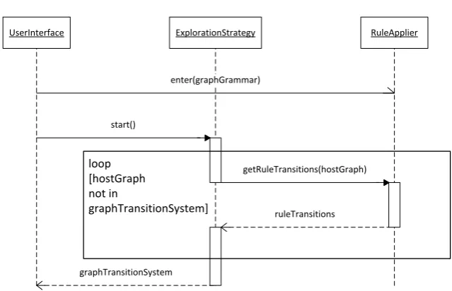
GROOVE is an open source, graph-based modelling tool, written in Java and in development at the University of Twente since 2004 [26]. It has been applied to several case studies, such as model transformations and security and leader election protocols [6]. A UML sequence diagram for GROOVE is shown in Figure 2.11, depicting a GG exploration to a GTS.

The tool functions as follows:

1. A graph grammar is given as input to a RuleApplier component, which determines the possible rule transitions.

2. The user selects an ExplorationStrategy from a list of possible strategies. This strategy explores all possible host graphs and rule transitions. The possible rule transitions from the initial graph state are obtained from the RuleApplier and a rule transition is chosen, based on the exploration strategy. The target host graph of the chosen rule transition is again given to the RuleApplier until no more new host graphs can be explored.

(24)

UserInterface ExplorationStrategy RuleApplier

enter(graphGrammar)

start()

graphTransitionSystem

getRuleTransitions(hostGraph)

ruleTransitions loop

[hostGraph not in

[image:24.595.141.461.97.303.2]

graphTransitionSystem]

Figure 2.11: GROOVE sequence diagram

2.5.3 GROOVE visual elements

Labels and ags Nodes in GROOVE have several kinds of labels: regular labels, type labels and ags. Figure 2.12 shows a node with a type label (bold), two ags (italic) and two regular labels. Nodes in GROOVE can have one type, indicated by the type label. Typing is not explained further in this report1_{. A node can have multiple regular labels and ags.}

Type ag1 ag2 label1 label2

Figure 2.12: GROOVE labels and ags

Rule node matching Nodes in a rule graph in GROOVE can also match the same host graph node, by connecting them with an equals `=' labelled edge. This means that any images of both nodes have to be the same. Figure 2.13a shows an example of this. Nodes in a rule graph in GROOVE can also explicitly not match each other, by connecting them with an not-equals `!=' labelled edge. This means that any images of both nodes cannot be the same. Figure 2.13b shows an example of this.

node1 = node2 (a) Matching rule nodes

node2 node1 !=

(b) Non-matching rule nodes

Figure 2.13: Node matching in GROOVE rule graphs

Colors Rule graphs in GROOVE combineLHS,RHS andNAC into one rule graph. The colors on the nodes and edges in GROOVE rules represent whether they belong to the LHS, RHS or NAC of the rule. See Figure 2.14 for an example.

(25)

1. normal line (black): This node or edge is part of both the LHS andRHS. 2. dotted line (red): This node or edge is part of theNAC only.

3. thick line (green): This node or edge is part of theRHS only. 4. dashed line (blue): This node or edge is part of theLHS only.

LHS_and_RHS NAC

RHS LHS

foo

bar

[image:25.595.236.361.185.240.2]

baz

Figure 2.14: GROOVE rule graph colors

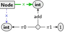
Variable nodes and terms Variable nodes in GROOVE are represented by their type: `int', `bool', `real' and `string' for integer, boolean, real and string variables respectively. Figure 2.15 shows two integer variable nodes and the constant integer node `1'. The diamond shaped node is a term node. It has two argument edgesπ0, π1 and a result edge `int:add'. The term represented

here is the addition of two integers, the rst one being an integer variable, the second being the number 1. When this rule matches a host graph, the target variable node of the result edge is set to the result of the term; in this case the image of the rst variable node plus one.

Node

int

1

x

π0 π1

[image:25.595.249.353.378.431.2]

add

Figure 2.15: Terms in GROOVE rule graphs

Term shorthand notation A rule node with an edge to a constant is shortened to a label on the node. Figure 2.16a shows a node with an edge labelled `x' to the constant `1'. Figure 2.16b shows the shorthand notation of this edge as the label `x = 1' on the source node of the edge. Terms can also be shortened. The rule graph in Figure 2.15 can be shortened to the rule graph in Figure 2.17.

Node x 1 (a) edge to constant

Node x = 1

(b) shorthand notation

Figure 2.16: Constant shorthand notation in GROOVE

Wildcards GROOVE features wildcards that can match any label, or a label from a set of labels. Figure 2.18 shows an example of this. The edge on the left `Node' matches any edge on a node typed `Node'. The right `Node' matches any node typed `Node' with the ag `a' or `b'.

(26)

Node

x := x+1

Figure 2.17: Term shorthand notation in GROOVE

Node Node_?[a,b]

?

Figure 2.18: Wildcards in GROOVE rule graphs

Quantication GROOVE supports quantication operations over nodes in rule graphs. Figure 2.20 shows a simple example. The `forall' operator here matches all nodes typed `Node'. GROOVE also supports the `exists' operator and nesting of operators, however this is out of scope for this report. The `forall' operator will be used in the model examples to perform operations over sets of nodes, such as in this rule: all self-edges labelled `x' on nodes typed `Node' are deleted from the host graph.

2.5.4 Example GROOVE graph grammar

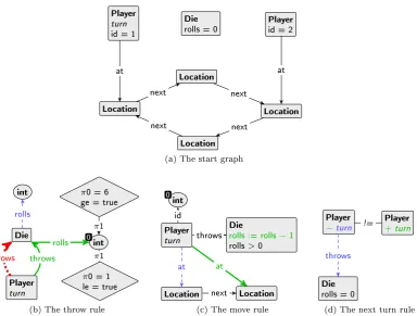
The running example from Figure 2.4 is displayed as a graph grammar, as visualized in GROOVE, in Figure 2.21. Figures 2.21b, 2.21c and 2.21d show three rules. Figure 2.21a shows the start graph of the system.

The rules can be described as follows:

1. 2.21b: `if a player has the turn and he has not thrown the die yet, he may do so.'

2. 2.21c: `if a player has the turn and he has thrown the die and this number is larger than zero, he may move one place and then it is as if he has thrown one less.'

3. 2.21d: `if a player has nished moving (number thrown is zero), the next player receives the turn.'

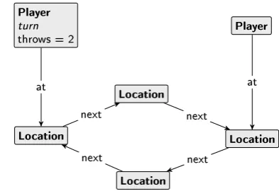
The graph is transformed after the rule is applied. The resulting graph after the transformation is the new state of the system and the rule is the transition from the old state (the graph as it was before the rule was applied) to the new state. Figure 2.22 shows the IOGTS of one ?throws rule application on the start graph. Note that the ?throws is an input, as indicated by the `?'. State

s1 is a representation of the graph in Figure 2.21a. Figure 2.23 shows the graph represented by

(27)

1 int 1 int 0 Node x x

π0 π1

add

(a) Rule graph

Node x = 1 (b) Host graph s0 s1 s2 add(1,2) add(2,3) (c) GTS

Figure 2.19: Rule transition parameters in GROOVE

Node

∀

@

x

Figure 2.20: An example of quantication in GROOVE

Die rolls = 0

Location Location

Location Player

turn id = 1

Location

Player id = 2

at next next next next at

(a) The start graph

Die int 0 int Player turn

π0 = 1 le = true π0 = 6 ge = true

throws throws rolls rolls π1 π1

(b) The throw rule

Die

rolls := rolls−1

rolls>0

Location Player turn Location int 0 at at next throws id

(c) The move rule

Player

−turn Player+turn

Die rolls = 0

!=

throws

[image:27.595.113.498.427.718.2]

(d) The next turn rule

(28)

s0

s1 ?throws(2)

Figure 2.22: The GTS after one rule application on the board game example in Figure 2.21

Player

Location Player

turn throws = 2

Location

Location _Location

Die

canThrow = 1 canThrow = 2 canThrow = 3 canThrow = 4 canThrow = 5 canThrow = 6

next at

Chapter 3

From Graph Grammar to STS

3.1 Requirements considerations

As described in seciton 1.5, the GRATiS tool needs to fulll three requirements:

1. A graph grammar must be used as the model; it must derive from the specication and be used for the testing.

2. It must be possible to measure the test progress/completion, by means of coverage statistics. 3. The solution must be ecient: it should be usable in practice, therefore the technique should

be scalable and the imposed constraints reasonable from a practical view point.

IOGGs In order to fulll the rst requirement, stimuli and responses have to be obtained from a GG. ATM uses an IOSTS, where the instantiated switch relations represent a stimulus to or a response from the SUT. GGs have no notion of inputs and outputs, therefore IOGGs have to be used as the model formalism. IOGGs can be explored to IOGTSs and the I/O labels of the IOGTS can be used to represent abstract stimuli/responses.

On-the-y vs. oine exploration The exploration of a GG can be done in two ways: on the y, rule transitions are explored only when chosen by ATM, or oine, the GG is rst completely explored and then sent to ATM. On-the-y model exploration works well on large and even innite models. However, coverage statistics cannot be calculated with this technique. The number of states (graphs) and rule transitions the model has when completely explored are not known, so a percentage cannot be derived. As coverage statistics are an important metric, the oine model exploration is chosen for GRATiS.

Data values An IOGTS can potentially be innitely large, due to the range of data values. This is a potential risk for the validation of the system. A model that is more ecient with data values is an STS. The setup of GRATiS is therefore to transform the IOGG directly to an IOSTS. This transformation should be done eciently to fulll the third requirement. Note that the second requirement is still met, because location and switch relation coverage can be calculated on the IOSTS.

(30)

1. Create an IOGG by assigning I/O types to the graph transformation rules of a GG 2. Create an IOSTS from the IOGG

3. Perform the model-based testing on the IOSTS

The rest of this chapter describes a declaritive denition for creating an IOSTS from an IOGG.

3.2 From IOGG to IOSTS

3.2.1 Variables in GGs

The location variables in an STS represent an aspect of the modelled system. For instance, if a system keeps track of the number of items in containers, the STS modelling this system could have integer location variables items1..itemsn. GGs do not have this kind of variables. The variable

nodes in rule graphs are used to match a value in a host graph, which is only available to that rule. A denition of persistent variables in GGs is needed in order to dene location variables from an IOGG. We deneVGGto be the set of GG variables in a GG.

Denition 3.2.1. GG variables

A GG variable is a tuplehla, lvi ∈ VGG, where:

• la is the variable label, which is part of an edge(za, la, za), where za is called the variable

anchor

• lv is the value label, which is part of a value edge: (za, lv, z), with z∈U.

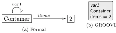
The item/container example modelled in a graph grammar could be a graph node representing a container with an edge labelled `items' to an integer node. This is shown in Figure 3.1a. The variable (var1,items)is now represented by this graph. Figure 3.1b shows the same example in

GROOVE. The variable edge is omitted here and the variable label is represented by the ag var1. This convention for GROOVE is used in the rest of this report.

Container items //

var1

2 (a) Formal

[image:30.595.188.382.505.560.2]

var1 Container items = 2 (b) GROOVE

Figure 3.1: Example of a GG variable

3.2.2 Graph exploration with point algebra

The IOGG cannot be directly made into an IOSTS, without using the IOGTS. To avoid the problem of a potentially innitely large IOGTS, the point algebra is used. Using the point algebra when exploring a GG has two eects:

1. The host graphs that dier only in value nodes are collapsed into one

2. The variable nodes in rule graphs can have at most one image in the host graph

(31)

3.2.3 The IOGG to IOSTS denition

First the declaritive denition is given, then each part of the denition is described in more detail.

Denition 3.2.2. IOGG to IOSTS

LetKbe an IOGG. FromKwe dene an IOSTSJ. The rst step is to exploreKusing the point

algebraP to an IOGTSOP. The elements ofJ can be obtained as follows: • W =G

• w0=G0

• L=VGG

• ı=φı, whereφı is dened below

• Λ =R

• I =V

• D=U, whereγ, ρare given by functions dened below

Locations The locations abstract from data values, exactly like host graphs do under the point algebra. Therefore, the set of locations inJ are the set of host graphs inOP. The initial location

inJ is also equal to the start graph ofOP.

Location variables GG variables were dened to have location variables in GGs. Therefore, it is no surprise that the set of location variables inJ is exactly the set of GG variables in OP.

This poses some constraints on creators/erasers for the variable anchors, variable edges and value edges. This is explained in detail in section 3.4.

Initialization function The initial value of the location variables is dened by the start graph. The start graph contains the GG variables and their initial values. This poses a constraint on the start graph, which is explained in section 3.4.

Denition 3.2.3. Initialization function

φı: (la, lv)7→z|(za, la, za)∈EG0∧(za, lv, z)∈EG0

Gates The gate of a switch relation represents the stimulus to or response from the SUT. In an IOGG, the rules represent the stimuli and responses. Therefore, the set of gatesΛ is equal to the

set of rulesR.

Interaction variables Interaction variables are used by the gates to represent a stimulus or response variable. The variable nodes in rule graphs are this representation. The set of interaction variablesI is equal to the set of variable nodes V. The arity of a rule is dened by the variable

nodes in theLHS of the rule:

arity(r) =|V ∩VLHS|

Switch relations A rule transition G−−→r,m G0 ∈ U is mapped to a switch relation (G−−−−−→r,φγ,φρ G0)∈D. Note that the set of locations is the set of host graphs, thereforeGandG0 represent the

(32)

gates, thereforerrepresents the gate of the switch relation. The functionφγ obtains the guard as

a term andφρ replaces theρfunction. These functions are dened in the next paragraphs.

Guard The guard of a switch relation restricts the use of the switch relation based on the values of the variables. In a GG, a rule is restricted by the terms. The variables used in the terms are interaction variables. Therefore, the rst part of the guard is constructed by joining the terms for each term node.

Denition 3.2.4. First guard function

φ1γ : Vz∈VLHS∩2T, t1∈z, t2∈zt1=t2

We apply this to the rule graph in Figure 3.2. This rule graph contains one term node, which in turn contains two terms. Formally, the rst part of the guard for this rule graph is:

(x1+ 1 =x1+ 1)∧(x1+ 1 =x2)∧(x2=x2)∧(x2>3 =x2>3)∧(x2>3 =true)∧(true=true)

Whent1=t2, the equation for this part is not useful, therefore it is omitted from now on.

int:x1 r1

b

o

d

a _/_/

r2 x1+ 1, x2

[image:32.595.248.354.595.678.2]

int:x2 x2>3, true

Figure 3.2: a rule graph

This rst part of the guard contains only the interaction variables. In an STS, the values forx1

andx2can be chosen such that the guard holds. However, the variable nodes cannot have just any

value; their value is determined by their image in the host graph. This image can be the value of a GG variable. Therefore we add a second part to the guard to link the interaction and location variables.

Denition 3.2.5. Second guard function

φ2γ : V(la,lv)∈VGG, z∈V∩VLHS|(za,la,za)∈EG∧(za,lv,m(z))∈EG(la, lv) =z

We apply this to the rule graph in Figure 3.2 and the host graph in Figure 3.3. The rule has a match in the host graph. The second part of the guard for this rule is:

(var1, b) =x1∧(var1, d) =x2

1 h1

var1

b

o

d

a _/_/

h2

1

Figure 3.3: a host graph

Denition 3.2.6. Guard function The complete guard is created by:

(33)

Update mapping When a value edge is erased from a graph and a new value edge is created with the same label and variable anchor, this inidicates an update for the corresponding GG variable. The update mapping for the switch relation represented by this rule transition should map the matched GG variable to the interaction variable represented by the target of the new value edge.

Denition 3.2.7. Update mapping function

φρ: (la, lv)7→z0|(za, la, za)∈EG∧(z, lv, z0)∈ERHS∧m(z) =za

This poses some constraints on the eraser/creator edges for value edges, which are explained in section 3.4. These constraints ensure thatφρ is bijective.

3.3 Rule priorities

Rule priorities are not taken into account in the denition above. First, we show why the denition above does not work with rule priorities. Then we show a method of including rule priorities in the IOSTS.

We apply the denition to the GG in Figure 2.9. We assume the rules both are stimuli, i.e. each is a I/O transformation rule(r,input), whereris the respective rule. All host graphs explored by

this GG are isomorphic under the point algebra, so they represent the same location. The IOSTS obtained from this IOGG is in Figure 3.4, withı={x7→25}. This IOSTS is wrong, because the

`?sub' switch relation can be taken from the start, whereas the `?sub' rule in the IOGG cannot be applied to the start graph, because it has a lower priority than the `?add' rule.

l0

?sub|x >10|x:=x−10

?add|x <30|x:=x+ 10

S

Figure 3.4: A wrong STS transformation of the graph grammar in Figure 2.9

The solution is shown in Figure 3.5. The negated guard of the `?add' switch relation is added to the `?sub' switch relation. The optimized guard for this switch relation is `x >= 30' of course, but this shows the main principle: for a rule transition u and a set of rule transitions U with

higher priority rules and the same source graph as u, the negated guard of the switch relations

represented by U must be added to the guard of the switch relation represented by u. In the

example, the `x < 30' guard is negated to `!(x < 30)' and added to yield the `x > 10 && !(x < 30)' guard.

l0

?sub|x >10 && !(x <30)|x:=x−10

?add|x <30|x:=x+ 10

S

Figure 3.5: A correct STS transformation of the graph grammar in Figure 2.9

(34)

all isomorphic graph states under the point algebra. Therefore, rule transitions with lower priority rules do not exist from that graph state and the respective switch relations also do not exist.

3.4 Constraints

In order for the denition in section 3.2 to work, four constraints are made for the IOGGs used in GRATiS. This section describes those constraints.

GG variable persistency All location variables in an STS are initialized to some value and no new variables are added. In a GG, it is possible to erase and create new variables in the transformation rules. Therefore, we pose the following constraints:

• All GG variables must be present in the start graph

• Variable anchors and variable edges cannot be erased or created

• A transformation rule may erase a value edge if and only if it creates a new edge with the

same source node and label as the erased value edge. The target node of the new edge must be a value node of the same sort as the target node of the erased edge

Unique GG variables The GG variables to location variables mapping has to be bijective. The previous constraints ensure the GG variables are always present, however they do not ensure their uniqueness. Therefore, we pose the following constraints:

• The variable labels have to be unique; there cannot be two variable edges with the same

label in the start graph

• The value labels for the value edges with the same source node have to be unique; there

cannot be two edges with the same variable anchor with the same label in the start graph

No GG variables in NACs In graph transformation rules, it is common to create restrictions on data using aNAC. For example, the rule graph in Figure 3.6a as aNAC expresses that the rule cannot be applied when the system is in state `done'. When using the point algebra, a problem occurs when a value edge is part of a NAC. The rule containing such a NAC will never match any host graph, because:

(a) the value edge is present in every host graph as stated in the previous constraints

(b) the target value node of the value edge will always be an image of the target variable node of the pre-image of the value edge. This is assuming the variable node in theNAC is of the same sort as the value node, otherwise the NAC would never have a match, because of the constraint on the sort of the value node of a value edge. Such aNAC would add nothing to the rule.

system

var1

S

status

“done”

(a) GG variable inNAC

system

var1

S

status

string:x x= “done”, f alse

(b) GG variable inLHS

(35)

Therefore we pose the following constraint: ANAC may never match the value edge and value node of a GG variable.

The correct way of modelling the example when using the point algebra is shown as theLHS of a rule in Figure 3.6b. Under the point algebra, both termsx= “done” andf alseevaluate to the

same boolean value. Therefore, an image for this term node can always be found, when the term node is in theLHS of the rule.

The guard of the switch relation will be (x= “done”) = f alse. This leads to a case where the

guard of the switch relation can never be satised. The following paragraph describes such a case.

Data constraints in node creating rules A case where a guard can no longer be satised is shown in Figure 3.7. This gure shows the LHS and RHS of a rule in the container-items example. The rule adds an item to the container unless it is full, i.e. has ve items. If an item is added, a new node labelled `new' is created in the host graph. Under the point algebra, this rule always matches the host graph and thus this rule creates an innite number of nodes. Therefore, the exploration never ends. This means that an IOGG with such a rule has an innite number of graphs and the corresponding IOSTS has an innite number of switch relations. However, the guards of the switch relations can no longer be satised when the location variable corresponding to the GG variable(var1,items)reaches5.

The rules in an IOGG which create new nodes or edges and have constraints on data should either:

• erase the same amount of nodes and edges as it creates

• have a constraint on the created node or edge, e.g. the node to create is part of theNAC of the rule

The rst constraint guarantees the exploration halts. The second constraint is only a guarantee if the node is the only element in theNAC, otherwise it is possible that theNAC does not match the graph even with the node in it.

container

var1

items

x1<5,true

int:x1

(a) LHS

container

var1

items

%

K K K K K K K K K

K new

int:x1 x1+ 1

(b) RHS

(36)

Chapter 4

Implementation

This chapter covers the general implementation of GRATiS. GROOVE and ATM, explained in section 2.5, are used for most of the functionality. Therefore, rst a general overview of the workings of GRATiS and how GROOVE and ATM t in the picture is explained in section 4.1. The added functionality is then explained in more detail in section 4.2.

[image:36.595.92.510.485.727.2]

4.1 General setup

Figure 4.1 shows a UML sequence diagram of GRATiS, depicting a general test run. This gure shows a combination of the UML sequence diagrams of GROOVE in Figure 2.11 and ATM in Figure 2.10. The interactions between GROOVE components and between ATM components as described in those gures is omitted where possible. The 'RemoteExploration' component replaces the 'ExplorationStrategy' in Figure 2.11 and the 'ATMInterface' component is added. These are briey included in the step-by-step explanation and explained in more detail later.

UserInterface RemoteStrategy RuleApplier

enter(IOGG)

start(host, port)

graphTransitionSystem

STSEngine TestManager

input(IOSTS)

start(depth)

result(verdict, trace) ATMInterface

setAlgebraFamily(point)

host:port(IOSTS)

(37)

1. The user enters an IOGG in the RuleApplier of the GROOVE tool. The input/output rules are dened by prexing the given rule names with '?' and '!'.

2. In the settings menu of GROOVE, the user sets the algebra family of the IOGG to to the point algebra, which is used by the RuleApplier.

3. The user selects the RemoteStrategy from the available strategies in GROOVE. This strategy gives input options to a host name and port number. The strategy is then started by the user. The communication between the RuleApplier and the strategy is omitted here, this is the same as in the GROOVE diagram. The result of the exploration is an IOGTS under the point algebra.

4. The RemoteStrategy creates an IOSTS in Java objects from this IOGTS with the method described in chapter 3. It then creates a message with the IOSTS and sends this message to the ATMInterface

5. The ATMInterface receives the message and gives the IOSTS to the STSEngine.

6. The ATMInterface starts the testing with the default `depth' parameter; making this cong-urable is not implemented yet. The communication between the TestManager, STSEngine and Adapter is omitted here.

7. The TestManager returns the test results to the ATMInterface. The test results are stored in a database and are viewable by starting the user interface of ATM (ommitted here).

4.2 Description of added functionality

This section covers in detail the added functionality to GROOVE and ATM.

GROOVE exploration strategy Figure 4.2 shows the class diagram of the added exploration strategy interface. The RemoteStrategy extends a SymbolicStrategy. The SymbolicStrategy has a closing exploration strategy, which is a strategy that explores all graph states and rule transitions, such as the BreadthFirstStrategy.

The user starts the RemoteStrategy with a host and port, as described above. This strategy starts a ClosingStrategy. This strategy explores the IOGG and noties the remote strategy when there are no more rule transitions to explore. The SymbolicStrategy implements the method described in chapter 3 to build the IOSTS in Java objects using the explored IOGTS from the ClosingStrategy.

RemoteStrategy

SymbolicStrategy ClosingStrategy

[image:37.595.225.378.558.661.2]

1 1

Figure 4.2: The class diagram of the exploration strategy interface

Model based testing with graph grammers