To the Question of Validity Grüneisen Solid State Equation
Vladimir Kh. Kozlovskiy
Jewish Scientific Society, Berlin, Germany. Email: [email protected], [email protected]
Received August 17th, 2012; revised September 19th, 2012; accepted September 27th, 2012
ABSTRACT
The first justified theory of solid state was proposed by Grüneisen in the year 1912 and was based on the virial theorem. The forces of interaction between two atoms were assumed as changing with distance between them according to in-verse power laws. But only virial theorem is insufficient to deduce the equation of state, so this author has introduced some relations, which are correct, when the forces linearly depend on displacement of atoms. But with such law of in-teraction the phase transitions cannot take place. Debye received Grüneisen equation in another way. He deduced the expression for thermocapacity, using Plank formula for energy of harmonic vibrator. Taking into account the depend-ence of atomic vibration frequency from distance between atoms, when the forces of interaction are anharmonic, he received the equation of state, which in classical limit turns to Grüneisen equation. The question, formulated by Debye is—How can we come to phase transitions, when Plank formula for harmonic vibrator was used? Debye solved this question not perfectly, because he was born to small anharmonicity. In the presented work a chain of atoms is consid-ered, and their movement is analysed by means of relations, equivalent to virial theorem and theorem of Lucas (disap-pearing of mean force). Both are the results of variation principle of Hamilton. The Grüneisen equation for low tem-perature (not very low, where quantum expression for energy is essential) was obtained, and a family of isotherms and isobars are drown, which show the existence of spinodals, where phase transitions occur. So, Grüneisen equation is an equation of state for low temperatures.
Keywords: Grüneisen Equation; Phase Transitions; Atomic Chain; Atomic Interactions
1. Introduction
The molecular-dynamical solid state equation, based on virial theorem, was derived by Sutherland [1], Mie [2], Grüneisen [3,4]. Another way of deriving, based on the Debye theory of heat capacity at low temperatures [5], which used the Plank expression for the energy of harmonic vibrator, was chosen by Ratnowsky [6], Eis-enmann [7], Grüneisen [8], Debye [9,10]. In classical limit the quantum equation of state turns to classical Grüneisen equation. But here arises a question, which Debye formulated in such manner: because an expres-sion of harmonic vibrator energy is used, can the Grüneisen equation be regarded as equation of state that describes phase transitions, which are non linear phenomena? In classical deduction of equation of state Grüneisen besides the virial theorem (which alone is insufficient to deduce equation of state) used some equalities that are strictly correct for forces that de-pends linearly from displacement of atoms. Debye tried to solve the formulated question, but, because he was based on relations correct for small anharmonicity only, the analysis cannot be regarded as complete. We em-ploy another way for equation of state deduction that
begins from variation principle of Hamilton, which can be a base for deriving of the virial theorem [11]. The approximations, used in solving of equations, are not burned to small anharmonicity. Here is given a brief account of equations deduction, which in details is published elsewhere [12]. The calculations for atomic chain show that Grüneisen equation is valid as equation of state for no high temperatures. The families of iso-therms and isobars illustrate the picture of phase tran-sitions in the chain.
2. The Basic Equations of Solid State
The deduction of virial theorem from Hamilton variation principle is briefly described below. The variation of mean time Lagrange function L is transformed as follows
2 2
1 1
2
1
1
2 1 2 1
1 1
2 1 2 1
1 1
d d
1 d 1
t t N
k k
k k k
t t
t
N N
k k
k t k k k k
L L
L L t q
t t t t q q
L L L
q t q
t t q t q t t q
q t
of movements equations, the second—for infinite time interval. The product of a coordinate with variable factor
represents a varied coordinate: qk qk, so k
,
k k k
q q q q .
These variations substituted in the left side of last Equation (1) give a relation
1 1
0
N N
k k
k k k k
L L q q q q
(2) If the kinetic energy W does not depend on coordinates
(in crystals rectilinear coordinates of atoms are used), it follows the virial theorem
_________ _________ ___ 1 1 2 N N k k
k k k k
U W
q q W
q q
NkT q (3)The represented variation procedure may be general-ised. The variable coordinates are represented in the form
, k k k k
q where k, k are variable parameters (further generalization of variation procedure is de-scribed in [12]). The variations of coordinates and ve- locities are expressed as qk k kqk,qk kqk and after substitution in (1) a relation follows
0
k k k k k
k k k k
L L L
q q
q q q
(4) So the equations are obtained
0 k L q
(5)
k k k
k k k
L L W
q q q
q q q
kT (6)
where the theorem about uniform distribution of kinetic energy is used. Further step in calculations consists in representation of coordinates as functions of time in the form
( ) k k k k
q s u t (7)
where sk are the mean values of coordinates, k is root mean square amplitude of vibrations, so the vibra-tion funcvibra-tions satisfy the relavibra-tions
u
0, 2
1k t k t
(8) If the kinetic energy depends only on velocities then (5) is represented as
0 k
U s
(9)
and
k
k k k k
k k k k U u L U
q s u
q q s u (10)
Introducing in (6) taking into account (7) and (9) we obtain k k U u u
kT (11)
If the system of atoms interacts with external corps, the positions of which are determined by means of coor-dinates i, the mean forces acting on the system are determined by expressions
a i i U A a
(12)
By shifting of the corps the forces produce a work, so the variation of energy by variation of all parameters is given by the expression
2 k k i
k k k i
H W U
N U U
k T s u A a
s u i
(13)Taking into account (9), (11) a relation will be ob-tained 2 ln N i i k k
H A a
k T u
T
(14)It can be seen that the quantity T which till now is only
the indication for mean kinetic energy, an integrant divi-sor for the quantity of heat is, hence proportional to ab-solute temperature. The expression for entropy is the follows 2 ln N k k
Sk T u
(15)We introduce a function of variables as an analogy of thermodynamic potential
__
ln k
i k
U kT u A a
i i (16) (items depending on temperature only are omitted). The condition of minimum Фby constant temperature leads to Equations (9), (11), (12) and allows to choose stable values of variables. In a crystal the mean values of dis-placements and amplitudes are equal for atoms belonging to the same sublattice, so the number of unknowns may be not great. Because in crystals the rectilinear coordi-nates are employed, the kinetic energy will not depend on coordinates.3. Anharmonic Vibrator with Two
Equilibrium Positions
an-harmonic vibrator with coordinate x and potential energy
of the form
2 4; 0,
2 4
c b
U x x c b0 (17) which is represented on Figure 1
It is necessary to determine mean time potential en-ergy, so it will be written
x s u t (18)
2 2 2 2 2
x s su t u t (19)
4 4 3 2 2 2
3 3 4 4
4 6
4
x s s u t s u t
su t u t
(20)
2 2 2; 4 4 6 2 2 4
x s u x s s u u 4 (21) where is put 30, because
t is an accidental function with zero mean value, so with equal probability receives positive and negative values, and in such man-ner behaves 3
.The mean value oft
4 is 3/2, if the
function is harmonic, but is greater, if on the path is potential barrier, which reduces the speed. Later we show what value of
t
4
is worthwhile to put in equations. So
2 2
4 6 2 2 4 42 4
c b
U s u s s u u
(22) The equations of state will be written as follows
2 20 ; 3 0
U
s c bs bu
s
(23)
2 2 2 4 4
; 3
U
u kT cu bs u bu k
u
T (24)
It follows two solutions 2 4 4 0 ;
s cu bu kT (25)
2 3 2 0 ; 2 2 9 4 4
cbs bu cu bu kT (26)
X U
Figure 1. Potential pit with two minima.
The first solution corresponds to vibrations above the potential barrier, the second to vibrations in left or right potential pit. If we put 4 = 3, then the left sides of
second equalities in (25), (26) differ only through multi-plier, consequently intersect the abscissa axis in the same point. For this case the Equations (25) and (26) are rep-resented graphically on Figure 2.
Parts of the curves that have physical meaning, corre-spond to positive temperature. Heating or cooling leads to transitions from one curve to the other, which is mani-fested in jumps of amplitude.
Braunbek [13] considered the phenomena of crystal melting, using the equation of sublattice motion. The potential curve was represented by a sinusoidal function of coordinate. The integration could be fulfilled with the help of elliptical functions. By low temperatures the at-oms moves in one of minimums of potential curve, by more high temperature—above the maxima. This corre-sponds to transition from crystalline to non crystalline state. On the Figure 3 is shown the calculated
depend-ence of the temperature from the energy of vibrations. The amplitude increases with energy, so it exists a possi-bility to compare the graphs, received with both methods of calculation. The graphs are similar, and the point of intersection of curves, describing finite and infinite movements (in our model also finite, but taking more place in the space) lies on abscissa axis. So, it is reason-able to accept 4 3.
A serious question arises by comparing our calcula-tions with calculacalcula-tions of Syrkin [14]. On the Figure 4 is
shown a form of potential pit: symmetrical double min-ima rectangular one.
Syrkin calculated the dipole moment in electric field for charged atom by means of formula for statistical dis-tribution, integrating over all space of the pit. It turned out that the dipole moment continuously decreases with
2 T
1
U2
W
[image:4.595.61.282.67.258.2]g
Figure 3. Relation between temperature and energy ac-cording [13].
[image:4.595.61.283.297.471.2]x U
Figure 4. Graph of potential pit according [14].
increasing temperature (as polarisability for thermal po-larization according to Debye formula). So, a discrep-ancy can be marked between dynamical and statistical calculations, but really this discrepancy is illusory, be-cause such question was considered in the literature. In the course of Frenkel [15] is discussed a metastable state with conclusion, that such state corresponds to a region of phase space, where the molecular system exists long time and can be observed, then for determination of phase integral the integration must be extended over this region. But Syrkin integrates over all space, which in-cludes both minima and potential barrier. This means that in no part of the space the atom delays for a long time, but jumps from one minimum to the other. Model of Syrkin corresponds to a hole in a crystal, where the atom is not bound tight to one minimum.
4. Equations of State of an Atomic Chain
It will be considered a chain of identical atoms situatedon x-axis, where atoms interact with nearest neighbours.
The extreme left atom with number 0 is fixed in the ori-gin and on the extreme right atom a constant force f
di-rected along the axis is acting (Figure 5).
Atom, which has the number k, interacts with left and
right atom with numbers k – 1 and k + 1, which are
placed on distances l lk, k1 from the considered. The energy of interaction for the whole chain is repre-sented by the sum
1
N k k
U U l
(27)If the mean time distance between neighbouring atoms is l—identical for all atoms, then the distance in moment t will be written as
k k
l l u t (28) where the mean square amplitude is written also as iden-tical for all atoms. The energy of interaction is further expended in power series with respect to amplitude and the order of derivative is marked by means of Roman numerals
2 2
3 3 4 4
1 2
1 1
6 24
I II
k k
III IV
k k
U l U l U l u t U l u t
U l u t U l u t
k
(29)
For taking the mean time value of (29) the relations (8) must be used and the mean time of (29) has the value
1
2 4
42 24
II IV
k
U l U l U l u U l u (30) For the function determined in (16) and calculated for one atom we receive, taking into account (30), an expression
2 44 1 2
ln 24
II
IV
U l U l u
U l u kT u f l
(31)
where f is a constant stretching force (hanging load). The
terms depending only on temperature are omitted. The conditions of minimum have the form
1
2 4
4 02 24
I III V
U l U l u U l u f
l
(32)
2 4
4 06
II IV
u U l u U l u kT
u
(33)
x N
1 K-1 K K+1
f
[image:4.595.314.538.612.729.2]If we neglect the terms containing fourth power of amplitude, an equation will be received
2 III I II U lf U l kT
U l
(34)
This is Grüneisen type equation. Now we deduce an equation with regard to fourth power of amplitude. We multiply (32) with IV
U and (33) with 1 4
V
U and sub- tract the second from the first, than it turns to be
2 1 1 2 2 1 0 4
I IV III IV II V
IV V
U U U U U U u
U f U kT
(35)
The Equation (33) will be solved with respect to 2 u
1
2
2 4
4
3 IV II II 2 3 IV
u U U U U k
T (36)
The radical is taken with positive sign, because the amplitude increases with increasing temperature and
which will be clear later. Expanding the radi-cal and retaining terms quadratic in temperature, we re-ceive. 0, IV U
4 2 2 1 6 IV II II kT kT u U U U (37)
Introducing in (35), we obtain the equation of state
4 2 3 2 24 2III II V III IV
I II
II
U U U U U
f U kT k
U U
T (38)
Further calculations concerning the transitions in the chain will be carried out retaining only linear in tem-perature term.
5. The Equation of State for Forces,
Changing with Distance According to
Inverse Power Law
The potential energy of two atoms, one of which is placed in the origin, other on the x-axis on the distance l
will be represented by means of a usual function
n mn m
U l
l l
(39)
which may be written in more convenient form
1 n 1 m
M
l U
n l m l
M
l (40)
This expression is mathematically equivalent to given in [16].
The minimum energy is displaced on distance lM, determined through equation
n m n m M M n m l l
(41)
The force constants may be expressed through lM,
1 1
, n
n lM M
n m
m
M
l
(42)
It follows the expression for the energy in the mini-mum M n m U nm
(43) Further we find
1 1
n m
I M M
M M
l l
U
l l l l
(44)
2 2
2 2
1 n 1 m
II M M M l n m U l l l l M l
(45)
3 3 3 3 1 2 1 2 n III M M m M Mn n l
U
l l
m m l
l l (46)
As can be seen, in the vicinity of the point M it must be II 0, because and the same is true for
U .
, nm IV
U
These values for derivatives of interaction energy sub-stituted in (34) give the Grüneisen equation for accepted law of interaction. We undertake now a mathematical investigation of this equation for the purpose to receive equations for isotherms and isobars and analyse their behaviour in order to discover transitions. As was noticed [17] the calculations are most simple for values n = 12, m =
6 that we introduce in above expressions and use the no-tation 6 M l q l
(47)
The expressions for energy and its derivatives are the follows
1 2
12
U q q
(48)
1
6 1
I
M
U q q q
l
(49)
1 3
2 13 7
II
M
U q q q
l
(50)
1 2 314 13 4
III
M
U q q q
l
The Equation (36) now turns to the form
1
6 1 13 4 7
13 7
M
q kT
f q q q
l q
(52)
As the multiplier in front of the bracket varies slowly with the length, we put
1 6 1
q and accept following approximate equation of state
1
13 4 713 7
M
q kT
f q q
l q
(53)
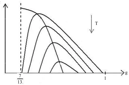
From this equation, as is usual in physical chemistry, a family of isotherms and isobars will be deduced.
6. Isotherms of the Atomic Chain
The expression in brackets, including the sign in front of it, consists of two items—The first is represented as a parabola, that goes to negative infinity intersecting ab-scissa axis in points q = 0 and q = 1, the top of which
arises above abscissa axis on 0.25. The second item is a fraction where numerator and denominator are linear functions of q and it aspires to constant negative value
when q goes to infinity, by diminishing of q also
dimin-ishes till the value q = 7/13, where the fraction turns to
negative infinity. So the function (53), when the tem-perature does not exceed definite value, is represented till this point by a curve with roots, lying between values of abscissa 0 and 1, and with top placed above the abscissa axis. By rising of the temperature the roots and the top coincide on the abscissa axis, and farther the chain can exist only under the action of negative (compressing) force. As it was noted in [17], the solid corps must resist to the action of stretching force, otherwise it is not a solid corps. The family of isotherms is depicted on the Figure 6. The physical meaning has parts of isotherms to the
right side of the top, where condition of stability 0
f q
is fulfilled [17]. In the top of the curves the transition in other phase takes place, but the structure of new phase is not described by the present considerations. It may be noticed in passing, that the branch of the curve to the left side of the top approaches the abscissa axis more abruptly, then that to the right side because the third derivative in the top is positive (when it is so, then in the vicinity of the top
top top
0
f f
q q
Expanding in series with respect to , we arrive at the formulated condition).
Each curve on Figure 6 is characterised by the
posi-tion and height of maximum and posiposi-tion of intersecposi-tion points with abscissa axis. The position of maximum is determined by the equation m
q
g T
f
1 13
[image:6.595.312.532.91.236.2]7
Figure 6. Family of isotherms of chain equation of state.
27 1 2 1 13 7
39 m m
kT
q q
(54)If this expression of temperature will be substituted in Equation (53), then the equation of the curve, connecting maxima of the isotherms (spinodal) will be obtained
1
1 2 1 13 4 13 7
39
M
m m
m m m
f l
q q
q q q
(55)
The right side decreases with increasing of the ab-scissa from the value7 13 0.538 , where the left side has the value 42 169 0.249 , till the intersection point with abscissa axis, where the top of the isotherm reaches it. As numerical calculation shows, here
0.745; m 0.0130 m
kT
q
(56)
The diagram (f, T) is represented in parametric form
by expressions (54), (55).
Now we determine the positions of the points, where the isotherm branches intersect the abscissa axis. Ac-cording to (53) one must put f = 0, then solve the
equa-tion
1 13
7
7
13 4
q q q
kT
q
(57)
We shall not solve this cubic equation to express the abscissa as a function of temperature, but shall confine us with consideration of solving procedure. The right side is a curve, intersecting the abscissa axis in the points q =
7/13 and q = 1, between them has a maximum. The left
7. The Isobars of Atomic Chain
From Equation (53) follows the expression for tempera-ture
7 13 7 1
13 4
M f l
kT q
q q q
(58)
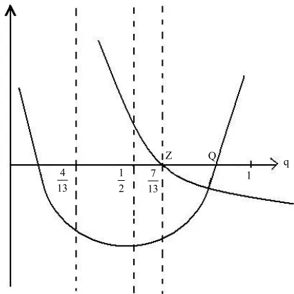
The right side is a product of a fraction with negative sign, whose numerator and denominator are linear func-tions of abscissa, and a quadratic function. The graphs of multipliers are represented on Figure 7 (the letter f on
vertical axis means function).
The temperature is positive, so physical meaning has the interval on abscissa axis, where the ordinates of both curves have the same (negative) sign that means interval between points, where the fraction and parabola intersect the abscissa axis. The first point is fixed; the second de-pends on the value of the force and may disappear (if parabola is placed above the abscissa axis). So, the fam-ily of isobars has the form, shown in Figure 8. Only the
part to the right side of the top, where T 0, q
have
physical meaning, because here the length of the chain increases with increasing temperature, what is designated as thermal dilatation (notation 47).
The position of the point Q, where parabola intersects
the abscissa axis is given by the expression
1 1
2 4
M Q
f l
q
(59)
With increasing force this point moves toward the point with abscissa 7/13 and coincides with it by the value of the force
q 1 f
Z Q
4 13
1 2
[image:7.595.316.534.82.289.2]7 13
Figure 7. Graphs of multipliers in Equation (58).
q
1 f
Q T
7
13 3 2
Q Q
Figure 8. Family of isobars of chain equation of state.
42 169
M f l
By this value the isobar disappears, and the system of atoms does not exist as regular structure.
For determination of maximum the expression (58) will be differentiated, and the result is
1
1 13 7 13 4 2 1
39
M
m m
m m m
f l
q q
q q q
(60)
This equation has the form of Equation (55). The value of temperature maximum on the curves, shown in Figure 8, we receive, if substitute the value of force (60) in (58),
where the value of abscissa is The temperature maximum is
. m q
27 1 2 1 13 7
39 m m
kT
q q
(61)and has the same mathematical form as (54). It is the equation of spinodale that joints the points of maxima on
Figure 8.
8. The Isobars Temperature—Amplitude
The initial equations are (37), (50), (58) and the problem consists in excluding the quantity q. This is made asfol-lows: Excluding the temperature leads to the equation for
q (here
1 3 1 q )
91 1 )
2
28 1
0w q w q p (62)
where w
u lM
2.M f l p
[image:7.595.68.281.499.712.2]form
28 1
2 91 1 w q
w R
(63)
where
2
28 1 4 91 1
R w w p
Introducing (63) in (37), leads to the expression for temperature
2
28 1
910 1 13
4 91 1
kT w
w R w R
w
(64)
The first multiplier turns to zero, when w = 0, the last
multiplier when p = 42/169 turns to zero also. When p =
0, the last multiplier is zero at w = 2/91. It can be proved
directly that for p laying between these extreme values
the last multiplier is zero at 2 1 169
91 42
w
p
(65)
So, the temperature has two roots with a maximum between them. The dependence of the temperature from the amplitude is shown in Figure 9. Physical meaning
has increasing part of the curve from zero to maximum. In the vicinity of the maximum the temperature is nearly constant, so the square of vibration frequency, which is proportional to the fraction, kT w2, diminishes with
nearing to the maximum. Such conclusion is formulated in Reference [18].
Gilvarry states that root mean square amplitude di-vided through mean distance between atoms at transition point has the same value for all substances with the same structure [19] and the same assertion is found in the arti-cle [20]. Such conclusion follows also from presented calculations. From (37) and (50) follows
1 2
2 3
13 7
M l kT u q
q q
(66)
With using the expression (47) for q this equality turns
to
[image:8.595.58.284.557.718.2]W P T
Figure 9. Family of isobars temperature—amplitude.
2
1
13 7
u kT
l q q
(67)
By means of equation of state (58), where is put f = 0,
this equation transforms to 2
1 1 7 13 4
u
l q
q (68)
To receive the value of q in the transition point, one
must differentiate (58) and the derivative equate to zero. Under the condition f = 0 definite value of q and
conse-quently definite value of fraction u l will be obtained.
9. Concluding Remarks
On the base of dynamic equations, that follow from va- riation principle of Hamilton, a thermal behavior of lin-ear chain of atoms, interacting with nlin-earest neighbors with forces, obeys inverse power law, and stretched with external force was considered. The mean potential en-ergy is developed in series with respect to the amplitude of atomic vibrations and only second powers were re-tained. This restricts the temperature from above, and the Grüneisen type equation of state was obtained. The fami-lies of isotherms and isobars were drowing, and spi-nodals are marked. So, Grüneisen equation is an equation of state, which describes phase transitions. This is the answer to the question, formulated by Debye: Is the Grüneisen equation an equation of state? The original calculations contain assertions, which are strictly correct for linear dependence of interacting forces from dis-placements of atoms, so no transitions can occur. It is a correct reasoning, and if we put in Equations (37), (38) the numerical values (56), we come to result that linear and quadratic in temperature items are nearly equal, so at such temperature quadratic terms cannot be ignored, and Grüneisen equation is an approximation useful for lower temperature. In a discussion about Grüneisen work Nernst expressed his opinion [3]:
“You all have received an impression, that we are so far, that can consider also the solid state from molecular- theoretical point of view, and one may hope that we soon receive a similar perfectly true theory also for solid state, that we for long time possess for gases.”
The Grüneisen equation in essential features turns into Mie equation, when in the fraction the terms, arises from attraction interaction, will be stroked out. So, the founda-tion for solid state equafounda-tion development is the Grü- neisen equation. The equation that takes into account terms with second potent of temperature will be essen-tially more complicated, than Grüneisen equation.
REFERENCES
Ex-perimental Introduction,” Philosophical Magazine Series V, Vol. 32, No. 199, 1891, pp. 524-553.
doi:10.1080/14786449108620220
[2] G. Mie, “To the Kinetics Theory of One-Atomic Corps,” Annals of Physics, Vol. 11, No. 8, 1903, pp. 657-697. [3] E. Grüneisen, “To the Theory of One-Atomic Solid Corps,”
Physical Magazine, Vol. 12, No. 22-23, 1911, pp. 1023- 1026.
[4] E. Grüneisen, “Theory of Solid State One-Atomic Ele-ments,” Annals of Physics, Vol. 39, No. 12, 1912, pp. 257- 306.
[5] P. Debye, “To the Theory of Heat Capacities,” Annals of Physics, Vol. 39, 1912, pp. 789-839.
[6] S. Ratnowsky, “One-Atomic Solid Corps Equation of State and the Quantum Theory,” Annals of Physics, Vol. 38, 1912, pp. 637-648.
[7] K. Eisenmann, “One-atomic Solid Corps Equation of State, according to the Quantum Theory,” Annals of Physics, Vol. 39, No. 16, 1912, pp. 1165-1174.
[8] E. Grüneisen, “Molecular Theory of Solid Corps,” The Structure of the Matter, Conference of Physics, Bruxeles, October 1913.
[9] P. Debye, “Equation of State and Quantum Hypothesis,” Physical Magazine, Vol. 14, 1913, pp. 259-260.
[10] P. Debye, “The Equation of State and Quantum Hypothe-sis with Supplement of Heat Conduction,” Lectures on the Kinetic Theory of Matter and Electricity, Leipzig and Berlin, B. G. Teubner, 1914, pp. 19-46.
[11] V. Fock and G. Krutkow, “Remarks to the Virial Theo-rem of Classical Mechanic,” Physical Magazine of USSR,
Vol. 1, No. 6, 1932, pp. 756-758.
[12] V. Ch. Kozlovskiy, “Dynamical Equations for Time- Averaged Coordinates at Thermal Equilibrium,” Soviet Physics Journal, Vol. 34, No. 4, 1991, pp. 353-359. [13] W. Braunbek, “Gratings Dynamics Theory of Melting
Phenomenon,” Physical Magazine, Vol. 38, No. 6-7, 1926, pp. 549-572.
[14] L. N. Syrkin, “To the Question of Temperature Depen- dence of Thermal Ionic Polarization,” Journal of Techni-cal Physics, Vol. 26, No. 6, 1956, pp. 1163-1165. [15] Ja. I. Frenkel, “Statistical Physics, Moscow,” Academy of
Sciences, Leningrad, 1948.
[16] Yu. M. Goryachev, L. L. Moiseenko and E. I. Shvartsman, “Parameters of Elastodynamic State of Dodecaborides of Rare Earth Metals,” Soviet Physics Journal, Vol. 34, No. 5, 1991, pp. 455-458.
[17] D. S. Lemon and C. M. Lund, “Thermodynamics of High Temperature Mie-Grüneisen Solids,” American Journal of Physics, Vol. 67, No. 12, 1999, pp. 1105-1108. doi:10.1119/1.19091
[18] F. Lindemann, “About the Calculation of Molecular Own Frequencies,” Physical Magazine, Vol. 11, No. 14, 1910, pp. 609-612.
[19] J. J. Gilvarry, “The Lindemann and Grüneisen Laws,” Physical Review, Vol. 102, No. 2, 1956, pp. 308-316. doi:10.1103/PhysRev.102.308
![Figure 3. Relation between temperature and energy ac-cording [13].](https://thumb-us.123doks.com/thumbv2/123dok_us/35524.503456/4.595.314.538.612.729/figure-relation-temperature-energy-ac-cording.webp)