publisher policies. Please scroll down to view the document itself. Please refer to the repository record for this item and our policy information available from the repository home page for further information.
To see the final version of this paper please visit the publisher’s website. Access to the published version may require a subscription.
Author(s): David Tall
Article Title: A Versatile Approach to Calculus and Numerical Methods Year of publication: 1990
Link to published version: http://dx.doi.org/ 10.1093/teamat/9.3.124 Publisher statement: This is a pre-copy-editing, author-produced PDF of an article accepted for publication inInstitute of Mathematics and its Applications following peer review. The definitive
publisher-authenticated version Tall, D. (1990). A Versatile Approach to Calculus and Numerical Methods. Institute of Mathematics and its Applications , 9, pp. 124 – 131. is available online at: http://dx.doi.org/
to
Calculus and Numerical Methods
David Tall
Mathematics Education Research Centre University of Warwick
COVENTRY CV4 7AL U K
Traditionally the calculus is the study of the symbolic algorithms for differentiation and integration, the relationship between them, and their use in solving problems. Only at the end of the course, when all else fails, are numerical methods introduced, such as the Newton-Raphson method of solving equations, or Simpson’s rule for calculating areas.
The problem with such an approach is that it often produces students who are very well versed in the algorithms and can solve the most fiendish of symbolic problems, yet have no understanding of the meaning of what they are doing. Given the arrival of computer software which can carry out these algorithms mechanically, the question arises as to what parts of calculus need to be studied in the curriculum of the future. It is my contention that such a study can use the computer technology to produce a far more versatile approach to the subject, in which the numerical and graphical representations may be used from the outset to produce insights into the fundamental meanings, in which a wider understanding of the processes of change and growth will be possible than the narrow band of problems that can be solved by traditional symbolic methods of the calculus.
The fundamental ideas are those of change, the rate of change, and the accumulation due to change. Symbolically these are represented by the function concept, the
derivative and the integral. In the calculus curriculum of the future, we need to broaden
our ideas of these three things to give a theory that applies not just to the beautiful abstraction that is traditional calculus, but also a theory that applies to the real world outside.
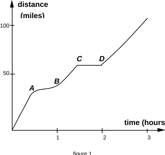
graph: fairly fast at all points except for the slower speed between A and B and the stop between C and D.
A B
C D
distance (miles)
time (hours)
50 100
[image:3.595.165.429.149.397.2]1 2 3
figure 1
This real-world example has the distance along the motorway as a function of time,
d=f(t), but it cannot be expressed in a neat symbolic way as a combination of
polynomials, trigonometric or exponential functions. So f(t) cannot be formally differentiated to give the derivative f'(t), yet the gradient of the graph still represents the speed.
On a computer, however, the graph might be drawn by remembering a large number of pairs (t,d) where d is the distance after time t, then the (average) speed from t1 to t2 can be calculate as the change in distance d2–d1 over the change in time t2–t1.
Thus it is natural to begin looking at numerical examples, and interpreting them graphically at an earlier stage than in a traditional curriculum, to use the graphical and numerical experiences as a transition to the usual symbolic theory. In this way, numerical methods should precede much of calculus, rather than being an afterthought to cope with cases where the symbolism fails.
concepts, such as the calculation of functions, ideas of range, domain and composition of functions, and graph-sketching, have been regarded as part of the pre-calculus syllabus. It is my belief that this view is a limited and mistaken one. If the concrete exploration of the theory of functions is seen as the first part of a broader calculus syllabus, then there are certain analogies with later parts of the syllabus which give the whole picture a greater coherence. To see this we need to dig a little deeper into the conceptual roots of the ideas.
Doing and Undoing
To obtain a “concept map” of a new curriculum which encompasses the calculus and numerical methods, it is helpful to begin with the fundamental idea of doing and
undoing, which permeates (or should permeate) the whole of mathematics.
In the early stages, subtraction “undoes” the operation of addition, division “undoes” multiplication. However, these forms of undoing are special in that they are precise inverses: subtraction of 2 is the unique way to undo the operation of addition of 2. When the operation of doing is a functional relationship, given x, find y=f(x), the “undoing”, given y to find x, need not be unique. Thus if y=x2, given x=2, there is a
unique value of y, namely y=4, but given y=4, there are two possible values of x, namely +2 and –2. Furthermore “doing”, in the case of finding y, given x, when
y=exsinx+x3/9, is just a routine calculation, whereas “undoing”, given y=3, say, and to find x to satisfy this relationship, requires a method of trial and error, or an algorithm which attempts to produce a sequence of improving approximations to the answer.
So often children get the idea that the solution of a problem always involves a straightforward operation (“is it a take away?”), that it would be valuable in mathematical education as a whole to concentrate on the operations of doing and undoing, where the first may be given by an explicit procedure, but the latter might involve some process of trial and error, or approximation algorithm.
the solving of equations can be done by trial and error, or by developing more powerful search techniques (bisection, decimal search, Newton-Raphson) or by iteration.
This leads to an essential sequence of stages in the development of numerical methods. First exploratory methods – investigations and inspired guesses – which can be used to get some idea of the nature of the required calculation. Then a simple, but effective method of solution which may be slow, but follows a clearly understood line of development. Finally a move to more powerful method that produces a quicker and more exact result using subtle theoretical refinements.
Representations
It is helpful to consider different ways of representing mathematical knowledge. Here we consider but three:
• numeric: where there is a given procedure to calculate a numerical
result,
• graphic: where the input and output of numerical calculations are
represented by a graph,
• symbolic: where the calculations are given in terms of algebraic
symbolism.
It is important to realize that these by no means exhaust all the possibilities. Other representations include verbal, say “multiply a number by itself to get the answer”, which is represented numerically by starting with an input, say 3, to get output 9,
graphically by the usual parabolic graph, and symbolically as y=x2. And many functions can be represented procedurally as a computer program, in this case the function may be written as a computer function in a form such as:
DEF FNf(x) = x*x
when PRINT FNf(3) would give the answer 9.
Simple programming allows numeric values to be calculated by more intricate methods, say the definition of the absolute value:
DEF FNabs(x): IF x>0 THEN = x ELSE = –x
or the definition of the factorial function:
where PRINT FNfactorial(1) will satisfy the conditional n=1, so output the value 1, but PRINT FNfactorial(2) will output the alternate definition 2*FNfactorial(1), where the FNfactorial (1) will output 1, so FNfactorial(2) will give 2*1. More generally PRINT FNfactorial(5) will give 5*4*3*2*1, and PRINT FNfactorial(n) will give the numerical value of n!.
Thus fairly elementary programming can be used to give functions more varied in nature than the traditional formulae of the calculus and we shall also find that such things as sequences of approximations that arise in calculating solutions of equations are naturally described in function notation which gives a new insight into the notion of convergence of sequences.
A concept map for calculus and numerical methods
A new approach to the calculus should concentrate on three aspects:
• change (the notion of function),
• rate of change (gradient of graph or derivative),
• cumulative growth (numerical or symbolic integration).
Representations:
Graphic Numeric Symbolic
Qualitative Quantitative Manipulative
Visualizing Estimating Formalizing
Conceptualizing Approximating Limiting
Concepts:
C h a n g e
doing: graphs numeric values algebraic
symbolism undoing: graphical numerical solutions inverse functions
solutions of of equations – (solving equations)
equations – sequences of symbolic
intersection numerical solutions
of graphs approximations
Rate of c h a n g e
doing: local numerical derivative
straightness gradient of graph
undoing: build graph numerical solutions solutions of knowing its of differential differential equations
gradient equations –antiderivative
Cumulative Growth:
doing: area under numerical area integral
under graph
undoing: know area know area – find FUNDAMENTAL
–find curve numerical function THEOREM
different possibilities?). This has been a rich area of new results in mathematical research and is far more interesting and realistic than learning a number of different tricks to obtain a few symbolic solutions.
I propose that new curriculum moves into the theory via a versatile combination of columns 1 and 2, with appropriate software available to give insight into column 1, and simple computer programming, or spreadsheet methods available for column 2.
In the new School Mathematics Project 16-19, a computer program called the Function
Calculator has been designed which allows students to make numerical computations
with functions without requiring programming in a computer language.
Change
The first part, on change, involves a number old friends, such as sketching graphs, but these may now be enhanced by computer software. For instance, graphs can be drawn easily by graph-packages, allowing concepts to be investigated such as the transformations which might move the graph y=f(x) to make it coincide with the graph of y=2f(x) or y=–f(x) or y=f(x+1), etc. Thus the symbolic effects of combining functions may be set in a context of experience based on the qualitative global graph-sketching carried out by a computer.
The numeric calculation of expressions leads to a genuine need to consider the nature of computer arithmetic and the propagation of errors, which at first can be performed simply using computer calculations. For instance, if a length d is measured as 2 units with an error e=±0.1, what would be the error in the result if this were divided by
c=1.2 where the latter is accurate to within an error f=±0.02, say. Clearly the lowest
estimate would be given by
d–e c+f
(with the smallest numerator and largest denominator) and the highest estimate is given by
d+e c–f .
By printing out these values the range of error in the result can be investigated.
and fairly good numbering on the axes, this can be a fairly accurate method of determining the answer.
Numeric solutions can be found first by trial and error (use a spreadsheet, or a computer program to calculate the values of f(x)–g(x) and search for where it changes sign). This will naturally lead to better search methods, such as bisection and decimal search.
Solution of the equation x=f(x) can be investigated iteratively by trying a solution x=x1. If x2=f(x1) and it happens that x2=x1, then a solution has been found. Otherwise, travel hopefully looking at x3=f(x2), x4=f(x3) etc, to see if the sequence of numbers x1, x2,
x3, ... homes in on a stable value.
This can easily be programed in a functional way. For instance, the functions:
DEF FNapprox(f$,x,n)
FOR k=1 TO n : x=FNf(x) : NEXT = x
DEF FNf(x)=EVALf$
in BBC BASIC will calculate the nth iteration of the equation x=f(x) starting at given value of x. Using this function, PRINT FNapprox("COS(x)",1,50) will print the 50th iteration of x=cosx starting at x=1. More interestingly, if we define a new function:
DEF FNa(n)=FNapprox("COS(x)",1,n)
then PRINT FNa(n) gives the nth term of a sequence, of which the following are the first few:
0.50302306 0.857553216 0.65428979 0.701368774 ...
whilst both PRINT FNa(100) and PRINT FNa(101) give 0.739085133.
Thus it is possible to talk about the convergence of sequences early in the course, long before the question of the convergence of series arises, and the nth term of the sequences concerned are more general than the simple algebraic expressions in n usually encountered. They can move in to a limit from above or below, they may converge or diverge slowly or quickly, and they are much more interesting to
investigate than simple formulae such as an=
2n2+1
concepts, but there is less room for the more obvious errors which are well-known to teachers.
Rate of change
Here the traditional approach used to be via an “intuitive” approach to the limit notion which has been shown by many researchers to be fraught with cognitive difficulties. Instead an approach based on numerical approximations, provided that it is done with
care, is more profitable. Doing it with care means calculating numerical gradients for
expressions of the form
f(x+h)–f(x)
h
where h is not too small. If it is too small (say 10–10) when the values of f(x) and f(x+h) are expressed as numbers (say to 8 or 9 decimal places) which are not affected by adding such a small number, then f(x+h)–f(x) will be zero according to the computer. Even worse, the calculation may have a tiny error which is nevertheless fairly large compared with h, so the expression becomes something about the same size as h on top, with an error of comparable size, leading to an incredibly inaccurate final result.
This is where the discussion of errors in the section on change has its first big payoff. Following the idea that each numerical calculation might be improved by a little subtlety, it is interesting to compute the “balance gradient” from x–h to x+h in the form:
f(x+h)–f(x–h) 2h
to see whether it is more accurate and when it may fail. Here a versatile combination of graphical and numerical results are unbeatable (until the student is able to get a more precise symbolic reason why the balance gradient gives a more accurate result using Taylor’s theorem).
The approach to the visual ideas shown by the graphics via magnification of graphs is well-documented elsewhere, together with the cognitive reasons why this is preferable over the old “intuitive” limit approach. (e.g. Tall 1987).
concern for less-able pupils, I believe this to be a serious conceptual omission which underestimates the versatile thinking power of the pupils and could lead to even greater conceptual pressure when even more new ideas are introduced in the second year.
The “undoing” of rate of change is the solution of (first order) differential equations – knowing the gradient – find the original graph. This can be attacked in a cognitive manner using the “solution sketcher” written for the School Mathematics Project 16-19. This is a computer program that, for a given differential equation, say
dy
dx = –xy
will calculate the gradient dy/dx for a graph using the formula on the right-hand side of the equation, (in this case –xy). As a pointer is moved round the screen, the gradient of a short line segment indicates the steepness of the graph through the point (x,y). It is easy to instruct the computer to leave a permanent mark for this line-segment, and by sticking them together, end to end, it is possible to build up an approximate solution to the differential equation.
It is also possible to give simple programs to provide numerical solutions, for example, the solution of the differential equation
dy dx =
1 1+x4
is given by
10 INPUT x,y 20 INPUT dx 30 dy=1/(1+x^4)*dx 40 x=x+dx : y=y+dy 50 PRINT x,y 60 GOTO 30
Functionally the general solution of dy/dx=f(x) where f(x) is given as f$ may be calculated as
DEF FNsol(f$,x,y,dx,n) FOR k=1 TO n
dy=EVALf$*dx:x=x+dx:y=y+dy NEXT
=y
to find the y-value of the solution starting at (x,y), taking n x-steps each of length dx.
Thus
will print the numerical value of the solution of dy/dx=2*x starting at x=0, y=0, taking 20 steps of length 0.1.
At an appropriate time (which may be demanding for the less able students at an early stage), this may be improved by letting the general equation dy/dx=f(x) be expressed by typing the expression f$ for f(x),
defining
1000 DEF FNf(x)=EVALf$
then replacing the calculation in line 30 by
30 dy=FNf(x)*dy
and improving it either by the midpoint approximation
30 dy=FNf(x+dx/2)*dy
or the “balance approximation”:
30 dy=(FNf(x)+FNf(x+dx))/2*dy
which may be seen to relate to the mid-ordinate and trapezium rules later in numerical integration.
Thus differential equations can be investigated for the first time soon after the study of gradient and differentiation. Conceptually the complement of the act of differentiation is the solution of differential equations, not integration.
Cumulative Growth
Cumulative growth, represented by the area under a curve can easily be attacked by a combination of graphic and numeric approaches. Programs to calculate the area are short and easy to write. In fact powerful conceptual functions can easily be written that will give the area a functional concept, for instance:
DEF FNarea(f$,a,b,n) s=0: w=(b–a)/n : x=a
FOR k=1 TO n: s=s+w*FNf(x+w/2): x=x+w: NEXT =s
DEF FNf(x)=EVALf$
PRINT FNarea("SINx", 0, PI/2,50)
gives the area under y=sinx from 0 to π/2 in 50 steps.
The function definition:
DEF FNa(n)=FNarea("SINx",0,PI/2,n)
again gives a sequence of approximations, here homing in on the area under sinx from 0 to π/2.
Or the function definition
DEF FNA(x)=FNarea("SINx",0,x,100)
gives the approximate area FNA(x) from 0 to x using 100 strips.
Again numerical area computations, combined judiciously with looking at pictures given by flexible software, can give great insight into conceptual ideas. For example, what happens to the area FNA(x) when x is negative? What happens to FNarea(f$,a,b,n) when b < a, or when the function is negative ? Investigate.
Following the earlier enunciated precepts that numerical approximations can be investigated to see if they can be subtlely improved, it is interesting to calculate, say the midordinate area M and the trapezium area T for the area under sinx from 0 to π/2 using the same number of steps. One overestimates, one underestimates. The errors are in an interesting proportion, namely
M = A+E, T=A–2E
where A is the true area and E is the approximate error for the midordinate. By attempting to cancel out the errors by taking
2M+T 3 =
2(A+E)+A–2E
3 = A,
we get a much better approximation for the error in the form 2M+T3 which simplifies to give ... Simpson’s rule...
the way for the theoretical introduction of Riemann sums, should this ever be studied in a later course.
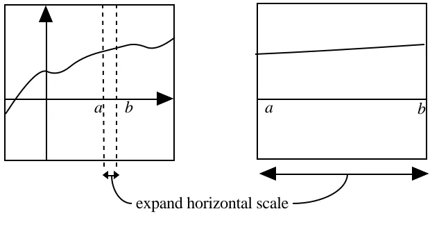
If a thin strip of a graph picture is stretched horizontally whilst the y-scale is unchanged, an interesting picture appears (figure 2).
a b a b
[image:14.595.142.452.163.325.2]expand horizontal scale
figure 2
This pulls the graph out flat – the tinier the strip the better it approximates to a horizontal line when stretched horizontally. If the area is calculated from an earlier point
a to a variable point x as A(x), then the change by adding on the strip is clearly
A(x+h)–A(x) = f(x)*h (approximately),
giving
A(x+h)–A(x)
h = f(x) (approximately).
The tinier the value of h, the better the approximation, giving
A'(x) = f(x),
which is the FUNDAMENTAL THEOREM OF THE CALCULUS.
Looking at the numerical methods of solving differential equations and the numerical methods of calculating areas, it will be realized that these are actually carried out by the same processes.
Thus the deep structure linking the various concepts is revealed.
Further extensions
This is not, of course, the end of the study of a versatile approach to the calculus. A very natural extension is to look at approximations to curves other than linear ones – to pose the problem if a function f(x) is approximated not by a linear form y=mx+c, but a more general polynomial
f(x)=a0+a1x+a2x2+...+anxn+e(x)
where the error function e(x) is, hopefully, very small. By the usual differentiation argument, the coefficients are found to be those of MacLaurin’s series, and a similar argument gives Taylor series
f(a+h) = f(a)+f'(a)h + ... + f(n)(a)hnn! + ...
Once more, these can be graphed, to see how good a global fit they are, or programmed as functions. For instance the expansion to the nth power of x
e(x,n) = 1+1! + x x
2
2! + ... +
xn n!
can be programmed as
DEF FNe(x,n) : s=1: t=1 : FOR k=1TOn: t=t*x/k : s=s+t: NEXT : =s
By investigating, for reasonably small x (say |x|<10) it is easy to find a value of n=N such that the value of FNe(x,n) stabilizes and doesn’t change for n>N. Thus the series for the exponential function is once more approached as a sequence of values which converges to a limit.
Reference
Tall D.O. 1987: ‘Understanding the Calculus’, a compilation of six articles from Mathematics
Teaching, published by The Association of Teachers of Mathematics, comprising:
‘Understanding the calculus’, Mathematics Teaching, 110, 49–53.
‘The gradient of a graph’, 111, 48–52.
‘Tangents and the Leibniz notation’,112 48–52.
‘A graphical approach to integration and the fundamental theorem’, 113, 48–51.
‘Lies, damn lies and differential equations’, 114, 54–57.