PROCESS CONTROL SYSTEMS SYNTHESIS
USING RULE-BASED PROGRAMMING
A Thesis
submitted in fulfilment of the requirements for the Degree of
Doctor of Philosophy in Chemical Engineering in the
University of Canterbury by
C. J. Williamson
THESIS
-n~) lrJ-~). ' \jl)
I?
Acknowledgements
I would like to thank my supervisor, Dr Brian Earl, for supplying the generous support that has enabled me to complete this project. Thanks are also due to Dr Raj Gupta who assisted me early in the project to unravel the complexities of structural controllability which subsequently played an important part in this work. I am grateful to the University of Canterbury for providing me with welcome financial assistance in the form of a Canterbury Postgraduate Scholarship.
Abstract
Chapter 1 - Introduction ... 1-1
1. 0 Introduction ... I -1
2.0 Thesis Structure ... 1-2
3.0 Previous Research into Control Systems Synthesis ... 1-4
4.0 Previous Research into Control-in-Design Techniques ... I-9
5.0 Control Systems Synthesis Using Expert Systems ... 1-13
6.0 Conclusion- Piping and Instrumentation Diagram
Generation ... 1-23
7.0 Nomenclature ... 1-23
Chapter 2 - Distillation Control.. ... Il-l
1. 0 Introduction ... II -1
2. 0 Distillation Control ... II -1
3.0 Expert System For Distillation Column Control Systems
Synthesis ... II-20
4.0 Nomenclature ... II-28
Chapter 3 - Heat Exchanger Control ... III-1
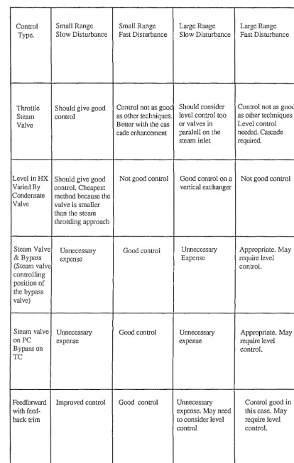
1.0 Knowledge Acquisition For A Heat Exchanger Expert
System ... III-1
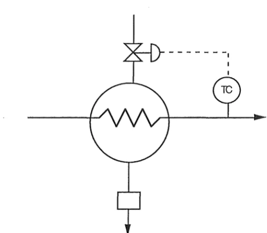
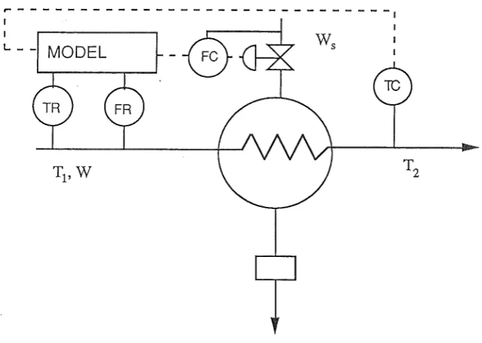
2.0 Heat Exchangers Without an Entire Stream Changing
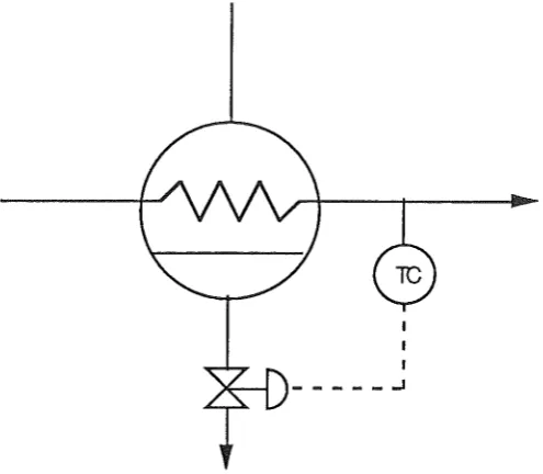
3. 0 Heat Exchangers With A Phase Change ... III -6 4.0 Expert System for Heat Exchanger Control System
Synthesis ... III-12 5.0 Nomenclature ... III-17 Chapter 4 - Reactor Control. ... N-1
1.0 Knowledge Acquisition for a Reactor Control Expert
System ... N-1 2.0 Continuous Stirred Tank Reactor Control ... . N-3
3.0 Plug Flow Reactors ... N-8 4.0 Fixed Bed Reactors ... ... N-11
5.0 Industrial Case Study of The ICI Oxo Reactor ... . N-12
6.0 The Reactor Control System Synthesis Expert System ... . N-14
7.0 The Program at Work ... . N-21
8.0 Nomenclature ... N-23 Chapter 5 - Structural Controllability ... .... V-1
1.0 Introduction ... V-1 2.0 State Controllability ... V-1 3.0 Structural Controllability ... V-3 4.0 Structural Controllability Applied to Control Systems
1.0 Whole Plant Control System Synthesis Using Expert
Systems ... VI-1
2.0 Preliminary Control System Synthesis Strategies ... VI-2
3.0 The Control Systems Synthesis Package ... VI-3
4.0 A Control System For a Complete Process ... VI-6
5.0 Conclusion ... VI-20
6.0 Nomenclature ... VI-21
Chapter 7 - Conclusions and Recommendations For Future
Work ... VII-1
1.0 Structural Controllability ... VII-1
2.0 Individual Unit Operation Expert Systems ... VII-2
3.0 The Whole Plant Control Systems Synthesis Program ... VII-5
4.0 Impact of Problems and Improvements in Expert
SystemsTechnology ... VII-6
References ... VIII-1
Appendix AI - Interaction With The Control System Synthesis
Package ... AI-l
Appendix All- Duff's Algorithm and the Johnston and Barton
Alternative ... AII-1
Appendix Alii- Rule Base For the Distillation Expert System ... AITI-1
Appendix AIV- Rule Base For The Heat Exchanger Expert
System ... AN-1
Appendix A V - Rule Base For The Reactor Expert System ... A V-1
Appendix A VI- TurboProlog Listing For The Distillation Expert
Appendix A VII - TurboProlog Listing For The Heat Exchanger
Expert System ... A VII-1
Appendix A VIII - TurboProlog Listing For The Reactor Expert
System ... AVITI-1
Appendix AIX - TurboProlog Listings of the Extra Programs For
Current steady-state process simulators have greatly increased the speed and efficiency of the development of Process Flow Diagrams. Chemical Engineers would benefit in the same way from a Computer Aided Design package to assist with generating completed Piping and Instrument Diagrams.
Despite the many theoretical methods available in the control science area there is no single and complete available solution to the problem of synthesising control systems for whole chemical processes and therefore no concrete basis from which to develop a computer program. Design activities rely on a significant experience factor and this element has largely been ignored especially in control systems synthesis. The recent emergence of rule-based programming allows this "experience" dimension to be added to software. Although there is previous work in the literature on expert systems for distillation column control systems synthesis there is very little published on programs for other unit operations or the whole plant problem.
In this project the problem of how to set up an expert system for whole plant control systems synthesis was addressed. As a preliminary step this required that expert systems for control systems synthesis for unit operations be written. The necessary knowledge to do this for distillation columns, heat exchangers and reactors was sourced from the literature and programs developed for each using a shell written in a version of Prolog. These programs were coordinated to work together and provide controllable solutions to whole process control problems using a matrix representation of the relationship between control objectives and manipulated vatiables developed in structural controllability analysis. This provided the framework for a prototype whole plant program. The operation of all the programs is illustrated using typical examples and their rule bases included in appendices to the thesis.
1.0 Introduction
Computer Aided Design has become progressively more important in the chemical engineering design office. The past few years have seen a proliferation of sequential modular steady-state process simulators and at least one equation-based package (SPEEDUP). As yet, however, there is no available software that an engineer can use to aid in the synthesis of control systems for whole chemical processes. There is a need for a package that allows the rapid synthesis of control systems for process alternatives thereby making the control aspect an integral part of the design process.
Rule-based programming, the major subset of expert systems technology, has grown to maturity in the last few years. This has allowed engineers to experiment with adding an "experience" dimension to their software. However, although this has lead to expert systems finding commercial use in areas such as process malfunction diagnosis and process control their use as synthesis tools remains a research area.
I-2
heuristics. It remains an unresolved question whether the solution to developing a package for control systems synthesis lies in an integration of presently available analytical methods and heuristics or in some as yet undiscovered theoretical technique, although the theoretical solution still seems a long way off.
As the solution to the problem seems closest using rulebased programming and already developed theoretical techniques this project aimed to explore the contribution to computer aided whole plant control system synthesis possible using rulebased programming. The research addressed a number of specific objectives within this area;
1) As heuristic rules have already proven useful in reducing the combinatorial difficulties associated with process design problems (Lien, 1987) to establish whether this was also true in control systems synthesis.
2) To identify relevant heuristic rules for control systems synthesis and investigate how best to translate them into current expert system software.
3) To investigate where heuristic methods should be used in preference to available theoretical methods and to research the integration of heuristic and theoretical methods into a single package for control systems synthesis.
4) To identify any parts of the control systems synthesis problem that can be handled effectively only by using heuristic methods.
5) As control systems synthesis knowledge is directed at a unit operations level to investigate how expert systems developed from this should be coordinated when an entire plant, rather than isolated units, is considered.
Knowledge on the control of three key unit operations; distillation columns, heat exchangers and reactors was acquired from the literature and organised into the appropriate form to write the corresponding expert systems. After they were completed in isolation these individual unit operation expert systems had to be coordinated together to solve whole plant control systems synthesis problems. Previous research into Structural Controllability Analysis, a technique previously considered for control systems synthesis, presented a possible solution to this part of the problem which allowed the development of a prototype package for whole processes.
2.0 Thesis Structure
Chapter 1 - The rest of this chapter is largely devoted to a literature review of previous research in the control systems synthesis and control-in-design areas. There is also an introduction to expert systems included to background terms and approaches used later in the thesis.
Chapter 2 - The first part of the chapter summarises the knowledge about distillation control found in the literature. It includes discussion of mass balance, single composition and dual composition control schemes. There are also details of further extensions to the basic regulatory structure of the column control system such as feed forward and cascade additions. The second part of the chapter describes the "shell" written in Prolog to implement this knowledge as an expert system and gives examples of the performance of the program.
Chapter 3 -The majority of the chapter describes the knowledge collected on heat exchanger control for two classes of exchanger. Heat exchangers without a phase change in a stream and those with a completely condensed heating stream. The second and smaller part of the chapter des<;:ribes the expert system for heat exchanger control developed from this knowledge. A similar programming style to the earlier work on distillation was used and examples from the two exchanger classes are included to demonstrate program operation.
Chapter 4- This chapter deals with the control of Continuous Stirred Tank, Tubular and Fixed bed reactors. The results of the literature survey and the consequent expert system are discussed. There is an example of the program at work on the problem of an exothermic CSTR.
Chapter 5 -A detailed review of Structural Controllability analysis makes up this chapter because of its importance in the development of the package for whole plant control system synthesis. Useful concepts and tools important in the final stage of the research, especially the work of Johnston and Barton, are highlighted and the fundamental necessity that a process control system satisfy structural controllability tests emphasised.
Chapter 6 - Describes the package for whole plant control systems synthesis using expert systems for unit operations coordinated by ideas taken from structural controllability. The solution provided by the program on an example process is included and compared with a control system for the same example derived from structural controllability considerations alone.
I-4
There are a number of appendices including English translations of the rulebases used in all the expert systems, the listings of the Prolog programs, the complete interaction between user and program that occurred when solving the whole plant problem in chapter 6 and a comparison between different mathematical methods required to provide the necessary structural controllability information for control system's synthesis.
3.0 Previous Research into Control Systems Synthesis
Control systems synthesis for whole chemical plants is a many faceted problem and the complete organisation of the solution method is as yet unresolved. The historical perspective is provided by Buckley (1964). He recommended material balance control to regulate plant production rate. The unit operations in the process are level controlled using either the product or feed streams. Any change in feed rate propagates through the plant. The unit operations quality control structure is superimposed on this to complete the control system. The assumption is that the feed changes are made infrequently and slowly while quality control disturbances occur fast and often. The material balance system doesn't therefore interact with the quality control system and both can be designed in isolation. This approach was adequate when plants were designed with little or no recycle, heat integration or other sources of interaction between unit operations. Now chemical plants are more integrated and energy efficient, significantly increasing the interaction between plant units. This change has emphasised the need to consider control early in the design process. The logical tools to accomplish this are computer programs that diagnose control problems in process designs and allow the rapid generation of whole plant control systems from process flow diagrams.
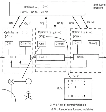
The first of the new generation of published work in this area was by Umeda et al (1978) who suggested a two level synthesis technique. The flowsheet is divided into unit operations and possible control systems for each are generated by analysis of the degrees of freedom available in mass, energy and momentum balances. These possibilities are screened using heuristic rules initially and finally through steady state and dynamic simulation to arrive at a collection of control systems that optimise the control performance of individual units and make up a first estimate of a control system for the flowsheet. This system is then analysed at the second level to eliminate conflicts between unit control schemes by applying heuristic rules with respect to the following;
-Location of flowrate control
In order to optimise the overall control performance of the process the revised control scheme is then passed back to the first level for reevaluation. The synthesis is complete when the proposed system passes through the procedure without being altered at the second level. Stephanopoulos has used a similar technique as an example in his text on process control (1984). A mathematical statement of the procedure is illustrated in Fig. 1.
Optimise 4> T (---)
( Cr,1i,-, Cr, nj,-, Cr, NK )
Cnj
r
r
Cr, nj
2nd Level problem
I
Optimize 11> (---) Opti.mize 4> n (--- ){Cnj}
r
-optimize <l> ( - - - )
I {
c
Nk}{ C1i}
I
_I
c. v.
1 0 - 0 0 1 0
M.V. 0
0 0 - - -1
C. V. :A set of control variables
M. V. : A set of manipulated variables
[image:15.600.88.501.237.675.2]I-6
The control performance functions at the unit level are labeled
<l>l·· ..
<J>n and at the plant level,<I>T·
Individual loops within the nth unit are Cn1··.
Cnm and the collection of loops for the nth unit is designated Cnj· This is a matrix of controlled variables vs. manipulated variables with entries where a manipulation is connected to a controlled variable in a loop. The revised control systems at the second level are Cr,nj and these are returned to the first level as shown.Control systems synthesis was subdivided into five aspects by Nishida, Stephanopoulos and Westerberg (1981);
a) A complete defmition of control objectives for the process b) The selection of controlled variables
c) The selection of a measured variable set d) The selection of a manipulated variable set
e) The design of the control structure (the interconnections between the measured and manipulated variables)
There are a number of techniques to aid with choices required in these five criteria. The identification of controlled variables, for example, can be divided into four distinct classes;
i) Operational constraints, usually in the interests of safety or process requirements eg. a pressure or temperature must be kept below allowable maximum values or within particular bounds to achieve a significant reaction yield, levels and flowrates must be controlled to adjust plant throughput.
ii) Product quality requirements eg. a 99% pure product.
iii) Environmental regulations that require that the level of contamination of
waste streams be kept below some maximum value.
iv) Economic considerations ie. which controlled variables should be used to decide the most profitable operating point for the plant.
variables kept constant by feedback. If the economic deterioration between the two is small the feedback alternative can be used. This simplifies on-line optimisation considerably.
Fisher, Doherty and Douglas (1988c) developed a similar but approximate approach to identify the optimisation variables as part of their steady state controllability analysis. If a variable hardly changes at the optimum operating conditions as steady state optimisation studies are made for a range of process disturbances then keeping it constant by feedback will approach the economic optimum. The optimisations are done by a short-cut rather than rigorous approach.
Govind and Powers (1982) pioneered an approach based on establishing all the possible measured and manipulated variables in two steps and combining these groups in a third to produce control structures for the process. The controlled variables must be identified before this procedure bt:<gins;
1) Possible methods for identifying the controlled variables are generated using a structural system array of the process. The array is a non-numerical representation of the mass, energy and momentum relationships between flowsheet variables in the Laplace domain. If a controlled variable appears in an equation in the array then all the variables apart from the controlled variable must be measured to allow calculation of it. The lower level variables then become the constraints and the process is repeated until no more branches can be added to the tree of measured variable set possibilities. This method is repeated for all controlled variables to identify the possible measured variable sets.
2) Manipulated variable sets are produced from the system cause and effect graph (a diagrammatic representation of the dynamic relationship between process variables). A directed edge points from one node to another if that variable affects the other. A variable is suitable to alter another if it affects it , and if it can be successfully screened through a set of heuristic rules and the constraint-variable transfer function (modeled as first-order plus deadtime) has an acceptable gain, time constant and lag.
3) The solution sets to the first two steps can be combined in different ways to produce a number of alternative control structures (feedback, feedforward and cascade) for any controlled variable and these can be grouped together to make up the control structure for the system. The method doesn't analyse further to establish which of the proposed structures is the best.
I-8
procedure, structural controllability analysis, that identified all feasible manipulated variable sets without error. Their method was refined by other researchers and is explained more fully in chapter 5.
The manipulated variable sets can be compared using measures derived from the transfer function matrix relating inputs to outputs, G. Singular Value Analysis has attracted recent research interest. The singular values are the square roots of the eigenvalues of the matrix G+G. A number of researchers have demonstrated that useful conclusions about control quality can be drawn using these quantities. Johnston and Barton (1985b), for instance, used the following to compare different manipulated variable sets for a double effect evaporator ;
i) cr(min)[I + GK]-1- this should be large for good quality control in the face of disturbances
ii) cr(max)[GK(I+GK)-1];:; cr(min)[GK(I+GK)-1] ;:;1 for good set-point tracking
iii) cr(min)[G] large to prevent manipulated variable saturation
iv) The process condition number,"(= cr(max)/cr(min), should be small to give stability in the event of model/plant mismatch.
I The identity matrix
G The plant transfer function matrix K The matrix of controller gains
Graphs of the four quantities (i - iv) vs. disturbance frequency are used to characterise and compare different control structures. This approach is suggested as an alternative to dynamic simulation.
Once the manipulated and measured variable sets are identified the interconnections between them must be found. The accepted approach in the last 20 years has been to minimise interaction between Single-Input Single-Output (SISO) loops and Bristol's relative gain array has proved a useful tool in this respect. More recently singular value decomposition (Lau, Alvarez and Jensen, 1985) has been investigated as a more powerful alternative.
requirements of the plant. There are few if any applicable theoretical techniques for selecting these additions. A comprehensive review of much of the work described in this section is provided by Stephanopoulos (1983).
4.0 Previous Research into Control-in-Design Techniques
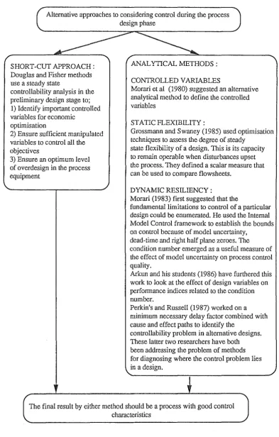
Recent research has tried to find tools that include control considerations in the design process as well as improving control system synthesis. There are two separate paths with the same ultimate goal, to synthesize as easy-to-control a design as possible. The first uses short-cut methods and the second has attempted to formulate a more analytical framework to attack the control in design problem. A summary of these approaches, discussed in the next few paragraphs, is illustrated in Fig. 2.
Fisher, Doherty and Douglas's procedure (1988a, 1988b, 1988c) belongs to the first as it is reliant on short-cut calculation techniques to screen possible flowsheets at a preliminary design stage. Quoting from the first paper in the series (1988a);
" At the preliminary stage of design, the optimum steady-state designs of various process alternatives are often uncontrollable ie. there are not enough manipulative variables in order to satisfy the process constraints and to optimise all the operating variables. Controllability can be restored by (1) modifying the flow sheet to add more manipulative variables, (2) overdesigning certain pieces of equipment so that the process constraints never become active for the complete range of process disturbances, or (3) ignoring the optimisation of the least important operating variables. The goal of a controllability analysis is to determine which of these alternatives has the smallest cost penalty"
In their second paper in the series they consider process operability. Quoting once again from their work (1988b);
" As disturbances enter the plant the fixed equipment sizes may prevent the process constraints from being satisfied or may prevent the operating variables from being adjusted to significantly lower the operating costs. Operability problems can be overcome either by an appropriate amount of flexibility or by developing alternative operating policies, and we want to determine the alternative that has the smallest cost penalty"
I-10
Alternative approaches to considering control during the process design phase
~---~~--
..., / ...,Douglas and Fisher methods use a steady state
controllability analysis in the preliminary design stage to; 1) Identify important controlled variables for economic
optimisation
2) Ensure sufficient manipulated variables to control all the objectives
3) Ensure an optimum level of overdesign in the process equipment
'
~/
ANALYTICAL .METHODS :
CON1ROLLED VARIABLES
Morari et al (1980) suggested an alternative analytical method to define the controlled variables
STATIC FLEXIBILITY:
Grossmann and Swaney (1985) used optimisation techniques to assess the degree of steady
state flexibility of a design. This is its capacity to remain operable when disturbances upset the process. They defined a scalar measure that can be used to compare flowsheets.
DYNAMIC RESILIENCY :
Morari (1983) first suggested that the
fundamental limitations to control of a particular design could be enumerated. He used the Internal Model Control framework to establish the bounds on control because of model uncertainty,
dead-time and right half plane zeroes. The condition number emerged as a useful measure of the effect of model uncertainty on process control quality.
Arkun and his students (1986) have furthered this work to look at the effect of design variables on performance indices related to the condition number.
Perkin's and Russell (1987) worked on a minimum necessary delay factor combined with cause and effect paths to identify the
controllability problem in alternative designs. These latter two researchers have both been addressing the problem of methods for diagnosing where the control problem lies in a design.
'
~•
The final result by either method should be a process with good control characteristics
[image:20.598.119.512.76.692.2]" By solving the optimum steady-state control problem in terms of the
significant disturbances and manipulative variables, we often find that the optimum
values of
some
of the operating and/or manipulative variables lie at constraints. If weselect these constrained variables as controlled variables, the resulting feedback system
will have near optimal performance without the need for measuring all the disturbances
or for calculating the entire optimum steady-state control policy on-line"
Their whole synthesis procedure .is summarised in Table 1. The discussed
methods make up level 1 of the complete approach.
level 1: steady-state considerations
la. Controllability. Identify the economically significant disturbances, and ensure that there are an adequate number of manipulative variables in order to be able· to satisfy the
process constraints and to optimize the operating variables over the complete range of the anticipated disturbances. lb. Operability. Ensure that there is close to the optimum amount of overdesign ,to be able to satisfy the process
constraints and to minimize the "expected" operating costs for the complete range of anticipated disturbances.
lc. Select the controlled variables. Select a set of controlled
variables so that the steady-state operating costs will be
essentially minimized. .
ld. Steady-state screening of control structures. Assess the amount of interaction in alternative control structures.
level 2: normal dynamic operation-small perturbations from
steady state .
2a. Inventory control. Ensure that the plant material and energy balances can be closed, and assess the need for intermediate storage capacity.
2b. Dynamic control. Assess the stability of the control structure alternatives, and ensure robustness. The analysis includes flow-sheet modifications (e.g., additional overdesign) to ensure process operability in the dynamic state.
level 3: abnormal dynamic operation
3a. Start-up and shut-down. Assess the need for special control systems for the start-up and shut-dov.'Il of the plant. 3b. Diagnostics and failure recovery. Ensure safe operation when equipment failures are encountered.
level 4: impl~mentation
4a. Distributed control. Organize the levels of local unit control, plant control, and supervisory control.
4b. Human interface. Ensure that the operators can operate the plant.
I-12
Swaney and Grossmann (1985) investigated a flexibility index which can be used to compare different processes. This scalar index, is a measure of the size of steady-state disturbance a design can withstand and still be operable. Unit operations are part of the control structure. If they saturate in the face of disturbances control is impossible. The approach is an analytical alternative to the Fisher and Douglas work on process operability but is far more computationally intensive.
There have been a number of research efforts aimed at measures of dynamic resiliency. These ideas frrst came from Morari (1983) who tried to develop a theoretical framework to find the bounds on control possible for a design regardless of .the controller type. He used the Internal Model Control (IMC) framework to come up with various measures indicative of particular control properties. He suggested three fundamental limitations that prevent implementing the plant transfer function inverse as the controller and realising perfect control (1) Non-minimum phase elements ie. deadtime and right half plane transmission zeros (these cause inverse response) (2) Physical constraints on manipulated variables (3) Model/Plant mismatch. In order to understand the control behaviour of non-minimum phase plants he factorised the transfer function matrix into two parts: G_G+ = G. The G. part is invertible and represents the best IMC controller while G+ becomes the closed loop transfer function. The optimum factorisation minimises an error measure (Integral Square Error) and represents the best control possible. The optimum factorisation for a process with time delays is a matrix with exponential terms on the diagonal representing the minimum achievable delay in output response. As an example, for a system with the optimum factorisation;
there is no control system that would achieve a setpoint with less than a single time unit delay in output 1 and a 3 time unit delay in output 2. The magnitude of these fundamental time delays are therefore a measure for comparing alternative flowsheets or a means to suggest design changes that improve their value. An example of a comparison between different control methods for heat exchanger networks using this approach can be found in the literature (Holt and Morari, 1985).
The minimum singular value is a measure of the tendency of the plant manipulated variables to saturate. Morari (1983) proved that
(1)
O'm(G) The minimum singular value of the transfer function matrix II u II max The norm of the vector of maximum input values
From (1) it is clear that the larger the minimum singular value of a process transfer function matrix for a multivariable system the less likely the manipulated variables are to saturate. This matrix quantity therefore represents a bound on the disturbances that a process can handle before an input reaches its maximum value.
The condition number emerged as a useful measure of the sensitivity of designs to mismatches between model and plant. The condition number, the ratio between the maximum and minimum singular values, measures the closeness to singularity of a matrix. As the condition number increases from 1 the matrix can be regarded as progressively less well conditioned until, if it is infinite, the matrix is singular.
Recent research on the "robustness" of control systems (Morari, 1983) has shown that the condition number is a quantitative measure of the sensitivity of the process to variations between the model used for controller design and the actual plant. More ill-conditioned processes rapidly lose control performance when operating conditions move away from the design point if an inexact model is used and may even become unstable. Barton et al (1986) describe the use of the condition number to screen ore recovery flowsheets. The results of the study, supported by dynamic simulation, showed that the condition number provided a convenient and accurate quantitative measure for the comparison of candidate flowsheets on the basis of control difficulty. Other studies of this type have been made with similar success (Perkins and Wong, (1985) and Levien and Morari (1987)).
The condition number concept has been extended by Arkun (1986) to define controllability performance indices that provide some diagnosis capability into which variables need to be changed to improve controllability. Russell and Perkins (1987) also recognised the failure of the developing techniques to diagnose exactly which elements of a design are causing controllability problems. They studied the "minimum necessary delay", a concept for grading systems with time delays, and combined it with cause and effect pathways in system matrices to identify the state variable and output responsible for it.
5.0 Control Systems Synthesis Using Expert Systems
I-14
eg. PID loops, cascade and feed-forward additions, overrides etc. This industrial approach to control systems synthesis consists of a number of steps. First determine the main flows, secondary flows and recycles, location of surge tanks, product streams with required purity specifications, turndown ratios, complex configurations and the availability of measurements and manipulations. Second the material balance controls are synthesised. Third, the product quality controls are developed for the various units often using plant data to determine the sensitivity of measurements to manipulations. Fourth, controls for secondary flows and temperatures are determined. Fifth, constraint controls and overrides are superimposed on the regulatory structure to maintain operation within feasible boundaries. Finally start-up controls are added. Choices at the different stages are made by experience rather than by analytical techniques. If any doubt exists at the end of this procedure it is resolved by dynamic simulation. This approach is possible because the situations where a particular control tool works are readily understood by the designer. Rule-based programming can turn this apparently fuzzy synthesis method into a usable CAD tool. The maturity of the technology means that this approach can produce useful programs now as long as the appropriate knowledge is available in an expert system.
5.1 Expert Systems
These are often also called Knowledge Based Systems (KBS) and the techniques used to write them rule-based programming. They are computer programs which use models of human reasoning processes in solving problems rather than the traditional algorithms. The typical expert system has 3 parts (fig. 3);
i) A knowledge base that contains the necessary knowledge to solve a problem (unchanged by inference). The commonest type is a collection of rules.
ii) Global data base that contains the facts about the problem to be solved (updated by input and altered during inference)
iii) Control structure that interfaces with the user and finds the problem solution using the knowledge available and the facts in the global database. In a rule based system this step uses backward or forward chaining
USER
I
USER INTERFACEl
CONTROL. STRUCTURE
IRULE INTERPRETER)
KNOWLEDGE
BASE GLOBAL
H
INPUTDATA DATA
• KNOWLEDGE RULES BASE
• INfERENCE RULES
IKNOWL.EDGE SOURCE! ·ISYSTEM STATUS!
Fig. 3 Typical Expert System Structure 5.1.1 Knowledge and Data Representation
There are two common kinds of knowledge representation in expert systems -"rules" and "frames" and one common data representation type- the "Object-Attribute-Value triple". The statement "Jill has red hair" can be formulated as object "Jill" has attribute ''hair-colour" with value "red". In a predicate logic representation this becomes "Jill (hair_ colour, red)". The predicate name is the object, the first argument the attribute and the second the value. PROLOG uses predicate logic as the basic statement form.
Rule-based systems use facts and rules to represent knowledge about an area of interest. The 0-A-V triples represent the facts. The rules have conclusions that can be drawn if the right facts exist. They take the form "IF antecedent THEN Consequent" where the antecedent must be satisfied by existing facts for the consequent to be true. These are known as IF_ THEN or production rules. The domain knowledge will often fall easily into this form.
I-16
the "Frame". A frame is a collection of Attribute-Value pairs that belong to the
particular object that gives the frame its name.The attributes in the frame are known as
"slots". A slot value can be already defined or ascertained from a procedure or
production rule called from the slot.
JILL : a_kind_of: @ WOMAN hair_colour - Red
eye_colour - Blue
Fig. 4 Frame Knowledge Representation
The a-kind-of link shows that Jill belongs to a class of objects called woman,
another frame. All the properties of the woman frame are said to be inherited by the Jill
frame. In some systems the frames can inherit slot values from more than one parent
frame. This is called multiple inheritance.
There is a further knowledge representation, related to the frame, called the
"semantic net". The domain knowledge is organised in a network of nodes and links.
WOMAN
Is Is
RED BLUE
The is-a link represents inheritance. The has-a link determines a node attribute.
5.1.2 Inference Procedures
The common inference procedures relate to rule based systems. The two types of computer reasoning for rule-based systems are forward and backward chaining.
5.1.2.1 Forward Chaining
Forward chaining is the inference mechanism used by one of the earliest and most well known of expert system tools, OPS5. The procedure begins with a set of facts about a problem stored in the database. The inference engine tries to match rule antecedents from the knowledge base with the facts. If a match is found the conclusion of the rule is added as a new fact to the database and the cycle is repeated. The inference procedure is completed when no more additions can be made to the database. The inference cycle has 3 stages - Match, Select, Execute. The match and execute stages are self explanatory but the select phase is more complex. After the match stage there may be more than one rule which has its antecedents satisfied by the facts. The select mechanism chooses the rule fired during that cycle. The selection criteria may be based on recency of facts, specificity of rule (most antecedents) or order of rules. The conflict resolution strategy may also be based on heuristics for prioritising rules (this represents "meta-knowledge" or rules about rules). If the following rules make up the data base;
1: if A andB then Y 2: if A thenD 3: ifD then E 4: ifD andY then Z
and the initial facts are A and B. The inference engine will cycle through the rules adding the conclusions of those with their conditions satisfied to the database. The result would be;
I-18
cycle 4. rule 4 is satisfied so Z is added to the database.
The final conclusion is Z and no more information is added in further cycles.
Rule order was used for conflict resolution.
5.1.2.2 Backward Chaining
Backward chaining is the reverse of forward chaining. The inference engine
starts with an hypothesised goal and tries to prove that it is supported by the facts in
the database and the rules in the knowledge base. The first step is for the system to
find a rule with a conclusion that matches the current hypothesis. The antecedent of
this rule may also be the conclusion of another. The procedure succeeds if the rule
chaining ends with a rule that has an antecedent satisfied by the facts. It fails if it
reaches a point where the antecedent of the current rule is neither a fact nor the
conclusion of another rule. If the procedure fails it should try another hypothesis to see
if this can be proven.
If the rules are the same as the previous example and the inference engine is
asked to prove if Z is true It would start with rule 4. If Z is true then D andY must be
true. Rule 2 has D as its conclusion and A must therefore be true. As there are no rules
with A as their conclusion it must be either a fact in the database or obtainable by
asking the user. The other branch of the "proof tree" concerns Y. Rule 1 has Y as its
conclusion so A and B must be true. If B was a fact then the backward chaining
would be complete and Z would be true. Issues of conflict resolution must also be
dealt with in a backward chaining system.
5.1.3 Explanation
A successful expert system should be able to explain its reasoning to the user
to allow a judgement on its soundness. The two common types of question that need to
be answered are "why" - why does the system need the information, and "How" - how
did the system arrive at the current conclusion. The "why" question is easily
implemented in backward chaining. An explanation facility can be a trace through a
goal tree. Using the above example again if the inference engine reached the point
where it was trying to establish A or B by querying the user if, in response, the user
asked the machine "Why" ie. why do you want to know that A is true, the machine
would reply with the rule "If A then D". If the user persisted and asked "Why" again
the system outputs the next level rule "If D and Y then Z". It is then clear how the
5.1.4 Knowledge Acquisition
This is the process followed by the "knowledge engineer" to go from the identified problem domain to an organised arrangement suitable for implementation as an expert system. Often the first step in this process is to locate an expert and get an explanation of how a problem is solved. In a series of interviews the knowledge engineer will try to distil the expert's knowledge into a usable form. This means identifying often used rules, the goals and subgoals followed by the expert in solving the problem, identifying the types of questions that the system should ask the user, and perhaps producing a "decision tree" to model the solution process. The process has no fixed procedure and is the bottleneck in the development of an expert system.
"Shallow" and "Deep" knowledge are terms often used to describe the results of the knowledge acquisition process. Shallow knowledge usually comes from interviewing and watching an expert work on examples and breaking this down into rules. The danger with this approach is that the system performance degrades absolutely if faced with a problem outside its scope. Deep knowledge models the real cause of the observed symptoms so that it is generic to the domain. Deep knowledge is more likely to be a causal model than rules, although rules may have some generic application.
5.2 Research on Control Systems Synthesis Using Expert Systems
The most pressing problem in developing an expert system for whole plant control is the structuring and organisation of the knowledge for solution. Although there are many texts available on process control the methods aren't stated in a form readily transferable to an expert system. Bristol (1980) pioneered a method he called "idiomatic control" that promises to be the basis for organising control knowledge. He recognised that most control problems were solved by experts using a set of 20-30 standard "idioms". These are control solutions that work time and time again. Common examples are PID loops, cascade control, feed-forward control but any experienced designer would have variations on these - their own set of idioms. Each of the idioms is appropriate in a particular situation and form generic building blocks to tackle new problems. Using a more complicated example, boiler level three term control is an idiom successful if the contents of a pressurised vessel are on the point of boiling, level control is difficult and material balance calculations are needed to achieve reasonable stability.
I-20
This concept was developed by Prassinos, McAvoy and Bristol (1984) who
tried to establish idioms and where they were successful by analysing operating control
systems. As an example cascade control will correct for flow upsets quickly by
cascading a slow controller to a flow loop. In subsequent work by Birky and MeA voy
(1988) idioms identified for controlling binary distillation columns were organised
using a knowledge representation technique called "Goal-Tree Success-Tree" (GTST)
which is shown in fig. 6.
Fig. 6 Goal-Tree Success-Tree Knowledge Representation
The GTST model identifies a top goal which is the primary objective of the
expert system. This goal is decomposed into sub-goals that must be satisfied for the
the top goal to be true. Each of these subgoals is decomposed into sub-subgoals
forming a tree with many levels. At the bottom level in the tree are specific conditions
that must be true to satisfy the lowest level sub goals. These conditions identify the
"success paths". A partial GTST model for distillation control system synthesis is
shown in fig 7. The authors claim that this knowledge representation is easily
tral(lsferred into a frame based knowledge base. The GTST also lends. itself to a
backward chaining inference procedure which is the more popular method for shell
design.
otTSRM!Nl! "RESr REdtJLATORY COtmmt.
SYST!lM RJR NORMAL OPERATION
I
I I
I
om~M!Nl!
I
Dfill!RMINEJ
VARIABLE PAIRINO VARIARI.E PAIRINO
FOR COMI'OStnON RJR MAT!lRIAI.
COtmlOL BALANCE COtmlOL
I I
I I I I I
DF.TIRMINE OETIRMINE OETIRMINE DETIRMINE DF.TIRMINF.
VAAIARLE VARIABLE VARIABLE VARIABLE VARIARLE
RJR DISTill.A T!l FOR Dam:>M FOR FOR RF.FUIX FOR COUIMN coMrosmoN COMPOSmDN PRESSURE DRUM LEVEL BASE LEVEL
COtmlOL COtmlOL COtmlDL COtmlDL COtmlOL
Prassinos et al also developed a handy idiom representation scheme which is readily transferable into frames. This provides a useful basis for a graphics interface with the user. This is the obvious communication method because engineers are trained to deal with PID's.
Distillation control system synthesis has attracted interest from other researchers as well. Umeda and Niida (1986) developed an expert system to design the regulatory system for column control. Their synthesis procedure is based around the model shown in fig. 8. Their expert system handles the first 4 stages in this procedure. It is implemented in CHIPS, a production system that uses forward chaining as its primary inference procedure .( An advanced version of OPS5). They went on to attempt a generalised system for use in whole plant regulatory control system synthesis (Niida and Umeda, 1986). In this work they used a frame based system (KEE).
S.l DEFINITION OF A PROCESS SYSTEM
t
S.2 DETERMINATION OF CONTROL OBJECTIVES
!
S.3 SYNTHESIS AND SELECTION OF POSSIBLE CONTROL LOOPS IN EACH UNIT
t .
S.4 ANALYSIS OF CONTROL LOOPS IN EACH UNIT AND COORDINATION AMONG CONTROL LOOPS
IN THE PROCESS SYSTEM
!
S. 5 DETAILED DESIGN OF EACH CONTROL LOOP
t
S. 6 CONFIRMATION OF CONTROL LOOP PERFORMANCE BY USING PROCESS DYNAMIC SIMULATORS
t
S. 7 CONFIRMATION AND ADJUSTMENT OF CONTROL LOOPS IN REAL PLANTS
Fig. 8 Control System Synthesis by Umeda and Niida
I-22
WHOLE PLANT CONTROL SYSTEM SYNTIIESIS STEP 1: STRUCTURAL ANALYSIS
When a process flowsheet has been selected the following procedure should be used to produce
a control scheme;
1) Identify the control objectives for the process. These arise from environmental,safety and product quality constraints. Although these should be relatively easy to identify problems arise if they aren't readily measurable and have to be represented by secondary measurements. Identify optimising control objectives using the Fisher and Douglas approximate technique or the more analytical tools of Arlrun et al.
2) Identify all possible manipulated variables.
3) Make a structural controllability analysis of the process. There are several requirements; i) Structural controllability matrices for all the units that make up the flow sheet.
ii) A coordinator matrix showing the relationship between all the manipulations and controlled variables Proceed by elinrinating controlled variables to produce a coordinator with full rank. This usually leaves a situation where there are more manipulated variables than control variables and a number of different manipulated variable sets therefore exist. Identify those sets that ensure structural controllability. The criteria used here could be either Morari's Integral Control Controllability or Perkin's Structural Functional Controllability.
STEP 2: ADVANCED DESIGN STAGE ALTERNATIVE ROUTE
The various manipulated variable sets can be turned into a control system using expert systems in a single step.
I) Analyse the points where alternatives exist (arising from the step 1)
using singular value analysis or additional information provided by Morari's _..,.. concept of the fundamental limitations to control quality. The important requirement here is a linearised state-space model of the plant. 2) If SISO loops are required then Bristol's Relative Gain Array or Lau and Jensen's Singular Value Decomposition technique may be of value in determining the control configuration.
1
STEP 3: FINAL DESIGN STAGE
At this stage the detailed control laws for the system can be produced and start-up,shut~down and emergency control systems introduced along with optimising and variable
control schemes (essentially using heuristic arguments)
The regulatory control structure is established then the necessary improvements such as feed forward, cascade, and other enhancements for step 3 can be added.
Design considerations can be mixed with control aspects and the system can call on the analytical techniques described in step 2
if required
FINAL RESULT
A completed Process and Instrumentation Diagram for the plant that can be checked for adequate control performance using dynamic simulation.
6.0 Conclusion - Piping and Instrumentation Diagram Generation
There is a recurring theme throughout this chapter. In both control systems synthesis and the consideration of control in design there are two approaches, the analytical one which struggles to invent theoretical methods with enough depth to address these complex issues and alternatively heuristic and short-cut approaches already used by engineers to produce workable designs. A diagrammatic summary of these alternatives when used to design .a control system for a process flow sheet is illustrated in Fig. 9.
The process begins with the determination of possible manipulated variable sets for the flowsheet using structural controllability analysis and then follows either a theoretical or heuristic path, based around expert systems, to develop a complete PID.
Expert systems may provide a CAD tool that offers a more complete answer in a single step than current theoretical methods. A well designed program would not only use rules but could call upon the "deep knowledge" represented by control theory to answer the design issues that require it. It would also attach importance to design factors that are not immediately concerned with control quality but are none the less vital for a good system design.
In this work, prototype computer programs that serve as the starting point for the development of a complete package for control systems synthesis based on the "alternative route" shown in Fig. 9 are demonstrated. The programs use already developed Ideas from structural controllability research to coordinate knowledge based systems that recommend control systems for the unit operations which make up the flowsheet. In one of the unit operations modules, written for distillation column control systems synthesis, Relative Gain Array calculations are used, if required, to improve the synthesis process.
7.0 Nomenclature
d =The vector of output disturbances G = The process transfer function matrix
Q+
=
The transpose of the process transfer function matrix I=
The identity matrixI-24
u =The vector of process inputs
Ys = The vector of steady-state process outputs
a( min)
=
The minimum singular value of the process transfer function matrixa( max)
=
The maximum singular value of the process transfer function matrix1.0 Introduction
This chapter begins with a discussion of distillation column control methods and ends with a description of how the bulk of this knowledge was translated into an expert system. The philosophy adopted in this work was that the program recommend likely schemes from the many available but allow the user to to make the final decision on which is the most suitable. This differs from other work (Umeda and Niida, 1986) where the program appears to make.only one recommendation. Control systems design is too complex an area for heuristic rules alone to decide the design but they are useful to screen out improbable options and reduce any subsequent workload.
The program can handle two product columns that operate with composition control on zero or one of the product streams, and also make recommendations for binary separations requiring dual composition control. The available knowledge could be deepened in two ways. The first would involve adding more recommendations on improvements to the regulatory structure, such as feed forward and constraint control. The second would widen its scope so it could handle more types of column, for example those with sidestream products.
2.0
Distillation Controlll-2
2.1 Mass Balance Control
This is a simple and cheap style of control for a two product column. The feed to the column and one of the product streams must be on flow control and the other product stream on level control to close the mass balance (Fig. 1 ).
r----
---1
I
I
I
I I
I
I
Fig. 1 Mass Balance Control
This type of scheme is a useful solution if the controlled product stream feeds a downstream column because it ensures a steady flow. If there are no disturbances expected in the input to the column (ie. the feed flow, composition and enthalpy are all constant) then this scheme is sufficient to ensure that the product stream compositions also remain constant. This is rarely the case in practice and this approach would hardly ever be successful.
2.2 Single Composition Control Schemes
Table 1. Composition Control AI ternati ves.
CONTROL
Method for
Case No. Overhead Reboiler Composition Free Composition Accumulator by Level by by
Control
1 D L B
v
Indirect temp*
2 D L
v
B V/F3 D
v
L B V/F4 D
v
B L Indirect temp5 D B
v
L Direct temp**
6 D B L
v
Direct temp7 L D
v
B V/F8 L D B
v
Indirect temp9 L
v
D B Mixed10 L
v
B D Mixed11 L B D
v
Indirect temp12 L B
v
D V/F13 B D L
v
Direct temp14 B D
v
L Direct temp15 B L D
v
Indirect temp16 B L
v
D V/F17 B
v
L D V/F18 B
v
D L Indirect temp19
v
D L B V/F20
v
D B L Indirect temp21
v
L B D Mixed22
v
L D B Mixed23
v
B D L Indirect temp24
v
B L D V/F*Indirect temp= Indirect temperature control scheme **Direct temp= Direct temperature control scheme
There are 24 possible schemes but most can be excluded by one of the following arguments;
1) A loop in the scheme has a large lag or deadtime associated with it, such as controlling reboiler level with reflux flow.
II-4
Fig. 2 Control of composition by varying boilup rate
I
feedflow
3) A scheme presents mass balance difficulties by not having at least one product stream on level control. These are options 9, 10, 21, 22 in Table 1, identified as "mixed"
These arguments narrow the choices down to fo~ widely accepted methods that fall in one of two categories, either "direct" or "indirect" temperature control schemes (fig 3). Within these two subgroups dynamic simulations (MCCune and Gallier, 1973) demonstrated the superiority of the indirect over the direct schemes when handling upsets in condenser duty. This is explainable because the indirect schemes have automatic reflux control ie. as the reflux is subcooled, top tray vapour flow reduces which in turn reduces external reflux through the level control loop. The internal reflux therefore remains constant and doesn't upset tray compositions. The responses of system 1 to upsets in energy or material balance (variations in feed condition) were also found to be the best. This scheme is recommended by other authors. Shinskey (1977), for example, is strongly in favour of indirect temperature control schemes, which he calls "direct material balance" schemes because of their insensitivity to enthalpy upsets. He goes funher to suggest that best control is afforded by using the smallest of the two product flows to control composition as this;
1) Reduces the absolute error in the material balance to the error in the smallest stream under flow control.
r---1
I
I
r • ,
I I
1£?
I
·---..!
'""
-
---~Indirect top temperature control
Direct base temperature control
Direct top temperature control
~+--~-_.\--,Q,
'....,.-'
I
Indirect base temperature control
II-6
This advantage is considered sufficiently important that he recommends a control structure which uses heat input to control reflux accumulator level and manipulates distillate rate to control bottoms composition when D/F << B/F.The accumulator level/heat input loop is not normally used by other designers because of the lag in response.
Fig. 4 A scheme recommended by Shinskey (1977) for base composition control when distillate is the s.maller product flow
Rademaker, Rijnsdorp & Maarleveld (1975) discuss indirect and direct temperature control. They listed criteria for choosing between the two different classes of schemes summarised as follows;
1) Temperature control on an indirect scheme is always slower than a direct scheme because the level control loop on the accumulator causes a delay before the change in external material balance affects column internal flows. A feed-forward addition to overcome this problem is described by Shinskey (1984), (Fig 5).
D*
L
D
The output to the reflux control valve is determined as the difference between the level controller output and the measured distillate flow.
2) The indirect temperature control scheme is logically favoured when distillate flow is too small to control accumulator level or bottoms level is too small to control column level.
3) In an indirect scheme the temperature controller introduces variation into the product flow which is undesirable if the stream feeds another unit operation requiring a steady feed.
4) The indirect scheme is more resistant to upsets in energy balance but contrary to the findings of other authors it is claimed that a direct scheme copes better with feed disturbances (this statement isn't supported by any evidence such as dynamic simulation).
5) In some cases there may be more significant interaction between level control using bottoms .flow and temperature control using heat input than when the loops are reversed (this is a disadvantage of indirect base composition control).
6) Indirect temperature control schemes can easily be converted to mass balance schemes especially if the temperature controller acts as the primary loop in a cascade configuration onto a product flow controller.
All the temperature control schemes function regardless of whether the composition is inferred from temperature or an actual analyser measurement is used. Accurate single composition control will keep both products on specification as long as there are no significant disturbances in feed flow and composition. In a case where accurate control of both products is important and disturbances upset operation the further complication of dual composition control is justified.
2.3 Dual Composition Control
The best configuration for dual composition control causes least interaction between the two composition loops. Shinskey (1984) details a method and selection criteria for this based on the calculation of the relative gain.
2.3.1 Interaction and Relative Gain
II-8
changes. This is divided by the steady state gain obtained with the other controlled variables constant (all other loops closed).
The relative gain array is a matrix of all possible relative gains between the manipulated and controlled variables in a system and it has the property that the sum of all the elements in each row and column is unity. A two by two array therefore needs calculation of only one of the four elements to complete the entire matrix.
The theory (after Stephanopoulos, 1984) on the use of the relative gain (A) as a guide to pairing variables is;
i) If A=O then the manipulated variable has no direct effect on the controlled variable and this doesn't represent a useful pairing.
ii) If A= 1.0 then the loop is completely decoupled from the others in the system. This is the ideal pairing.
iii) If 0 < A < 1.0, the gain increases when other loops are closed, and the smaller the A value the more significant interaction becomes and the less suitable the pairing.
iv) If A is< 0 then the loop gain changes sign when other loops are opened or closed. This leads to instability.
v) If A > 1.0, the gain reduces when other loops are closed, interaction reduces effectiveness.
2.3.2 Interaction and Dual Composition Control
Level and pressure control loops usually act much faster than composition loops. This means that only interaction between the composition loops needs to be taken into account. The problem is therefore simplified to calculating a number of 2 x 2 relative gain arrays.
In Shinskey's approach the alternative manipulated variables are the distillate flow (D), the vapour flow (V), the reflux flow (L), two independent ratios; reflux flow/bottoms flow (LIB) and boilup rate/bottoms flow (V/B) and the separation factor (S), defined by the equation;
S=
(
_ )nE
y(l-x) _ athe second part of the equation demonstrates that separation factor is fixed by controlling distillate flow/reflux flow (D/L). As the ratios reflux flow/distillate flow (LID), reflux flow/boilup rate (LN) and distillate flow/boilup rate (DN) are all dependent on D/L they are also options for separation control.
This makes a total of six independent manipulated variables available and control of any two will flx the end compositions of the column. Therefore there are 15 relative gain arrays. As these are 2 x 2 arrays they are completely characterised by calculating or measuring the first element in the array. A worksheet of these values can be evaluated for a particular column and used as a reference to make a selection.
Control y wi
Control ~ wi fh
t h t
D
-B
v
9/L
V/9
VID
-
VILD
I
Aov
Aol../1
A.,.fl
A OS
l LID D/VI D/L
ALO
-A so
ALv A sv
A..ue A SL/B
A LV/I A SV/B
Fig. 6 Relative Gain '\Vorksheet
There are gaps in the worksheet where pairings are unlikely or impossible. For example, D can't be used to control both x andy (this option is shown shaded in the worksheet) and neither can separation factor (the entire right hand bottom corner of the worksheet is missing because of this ).
II-10
2.3.3 Selection Criteria
Shinskey suggests some other factors that should be taken into account along with interaction when configuring the control system;
i) The smallest flow should be manipulated to control composition because this reduces the error in column material balance to the error in the flow of the smaller product flow.
ii) The accuracy of the material balance is also important when considering which ratio to use when controlling the separation factor. The smallest ratio should be used eg. ifD < L manipulate D/L (or, even better still,
DN
as V=L+D) and use L for accumulator level control. The ratio would be LID ifL <D.Considering these factors and the relative gain worksheet there are several commonly acceptable configurations
1) The top composition controlled by separation factor and the bottom composition by boil up rate/ bottoms flow (V /B). This is known as the SV /B configuration (fig 7) and should be used when Asv/b (the relative gain for the SV/B scheme) is in the range 1-5 and distillate, D, is smaller than B. This represents the closest thing to a universal solution to dual composition control as it has a fast response and the smallest relative gain of the group of options that have relative gains greater than 1.
In the SV
1B
scheme the top composition controller outputs the requiredDN
ratio which is converted to a set point for a distillate flow controller by multiplying this signal by the h~vel controller output (V= L + D). Changes in distillate flow are transmitted to reflux flow by subtracting its measurement from the output of the level controller (L=V-D) and using this as a setpoint for a reflux flow controller. The bottom composition controller outputs the required V /B ratio which is converted to a setpoint for a boilup flow controller by multiplying by the bottoms rate B.
This scheme is superior to the simpler SV (fig 7) configuration that has been used successfully in industry (Ryskamp, 1980) because it has improved interaction characteristics. The SV scheme in Fig 7 uses D/L as the ratio to control separation factor. This is slower than the
DN
choice because any change in distillate rate is only transmitted to the column when the accumulator level loop alters reflux flow. TheDN
Stt
SV/B
sv
8
Fig. 7 Top composition controlled by separation factor and bottom composition by V/B (SV/B) or by V (SV)
2) The top composition controlled by distillate flow and the bottom composition by boilup rate/bottoms flow 01/B). This is known as the DV/B scheme (Fig. 8) and is applicable when Asv/b > 5 and Adv/b (the relative gain for the DV!B scheme) is in the range 0.9- 1.0 and the distillate is the smallest flow.
Fig. 8 Top composition controlled by distillate flow and bottom composition by V/B (DV/B) or by V (DV)
ll-12
usually improves the relative gain. The major problems with this simpler scheme is a relatively sluggish response especially in the bottom loop and a failure to control if the top loop is left open. If this happens the heat input valve tends to saturate if there is a feed composition upset, such as an increase in the light components, because the material balance is fixed. The lights accumulate on the trays and finally collect in the base of the column. The boil up rate increases to maintain bottom composition but as the distillate remains constant the light components aren't easily removed and the heat input valve will be forced to open fully to maintain control.
3) Top composition controlled by separation factor and bottom composition by distillate. This is known as the SD scheme (Fig. 9) and is applicable when Asv/b > 5, D < B and Asd (the relative gain for the SD scheme) is in the range 0.9- 1.0.
Fig. 9 Top composition controlled by separation factor and bottom composition by distillate rate (SD)
This scheme includes the pairing of accumulator level with boil-up which isn't widely accepted because of the lags inherent in the column. The compromise is made here because the pairing of distillate, the smaller product flow, and bottoms composition improves the accuracy of the column material balance.
SB
Fig. 10 Top c