Parametric Iteration Method for Solving Linear Optimal Control Problems

http://dx.doi.org/10.4236/am.2012.39155 Published Online September 2012 (http://www.SciRP.org/journal/am)

Parametric Iteration Method for Solving Linear

Optimal Control Problems

Abdolsaeed Alavi1, Aghileh Heidari2

1_{Department of Mathematics, Payame Noor University, Tehran, Iran} 2_{Department of Mathematics, Payame Noor University, Mashhad, Iran}

Email: [email protected], [email protected]

Received June 13, 2012; revised August 7, 2012; accepted August 14, 2012

ABSTRACT

This article presents the Parametric Iteration Method (PIM) for finding optimal control and its corresponding trajectory of linear systems. Without any discretization or transformation, PIM provides a sequence of functions which converges to the exact solution of problem. Our emphasis will be on an auxiliary parameter which directly affects on the rate of convergence. Comparison of PIM and the Variational Iteration Method (VIM) is given to show the preference of PIM over VIM. Numerical results are given for several test examples to demonstrate the applicability and efficiency of the method.

Keywords: Parametric Iteration Method; Optimal Control Problem; Pontryagin’s Maximum Principle; He’s Variational Iteration Method

1. Introduction

Consider linear system described by

 

 

 

0 0 0

, ,

.

x Ax t Bu t t t

x t x

  





(1)

where are the state and control vector, respectively. are constant matrix and 0

,

n

x u

n n 

m



, n m

A  B

x is the initial state. The Optimal Control Problem

(OCP) is to find a control law which minimizes the quadratic cost functional

 

*

u t

   





0

1 1 _{d .}

2 2

f

t

T T

f f

t

T

J x t Sx t 



x Qx u Ru t (2)

where are symmetric positive semi-definite matrices and is symmetric positive definite matrix.

, n n

S Q Rm m

In general the problem can be transformed to the Ric-cati differential equation [1], although solving the RicRic-cati equation arised from OCP is not very simple. Another proposal for directly solving the OCP is discretizing the original problem and solving it numerically. Herein, the spectral collocation methods differ from other computa-tional methods in their special discretization at carefully selected nodes for example, the so-called Legendre- Gauss-Lobatto nodes. Then the differential equations of the OCP are approximated by algebraic equations [2]. Although these methods are flexible and for program-ming with computer are compatible, but they have their

weaknesses for instance they react quite sensitively on the selection of time-step size [3].

According to the classic optimal control theory, as pointed out in [4], by using Pontryagin’s maximum prin-ciple, we can obtain the following Two-Point Boundary Value (TPBV) problem

 

 

 

 

 

 

 

 

1

0 0

,

.

T

T

f f

x Ax t BR B t x t x

t Qx t A t t Sx t



  



  

 

  

 

 _

， (3)

and the optimal control law for OCP can be written as

 

 

* 1 T

u t  R B  t where is known as the

costate variable.

 

n t

 

Analytic solutions can rarely be found for such TPBV problem and authors often solve it approximately for example Yousefi, Dehghan and Tatari [5] applied He’s Variational Iteration Method (VIM) to find the optimal solutions. In this paper, we are going to solve (3) by use of the Parametric Iteration Method (PIM) with emphasis on preference of PIM over VIM.

2. Parametric Iteration Method

PIM is an approximation method for solving linear and nonlinear problems and at beginning it was proposed for solving nonlinear fractional differential equations [6], by modifying He’s variational iteration method [7]. The idea of PIM is very simple and straightforward. Consider the following differential equation:

 

0.

where A is a nonlinear operator

(5) where L denotes a linear differential

, t denotes the time, and

 

u t is an unknown variable. To explain the basic idea of M, we first consider Equation (4) as below:

 

 

 

, 0.

Lu t Nu t g t t

PI

operator with respect to u, N is a nonlinear operator with respect to u and g t

 

is the source term. We then construct a family

of iterative formulas as:

 

 

1

n n

L u  t u t hH t A u

 

 n

 

t  (6)

where and denote the so-ca ter and



Accordingly, the successive approximations 0

h

rame

 

0

H t 

auxiliary

lled auxil- iary pa function respectively. Now by use of 1

L which is a weighted integral operator, we

have:

 

 

1



 

 

1 .

n n n

u t u t L hH t A u t 

 

n u t ,

th 1 will be readily obtained by choosing the zero mponent u t0

 

satisfying the general property

 

0

 

0 , .

n

u t u t  n 

n co

(7) One logical guess for u t0

 

inear can so

w

3. Solution of Optimal Control Problem via

In solving the OCP described by (1) and (2), the PIM constructs the following sequences to directly

ap-be stablished by lving its corresponding l homogeneous equation

 

0 0

L u t_ _ . Another choice is u0

 

t u0 according

to the i ondition. Otherwise it ca freely chosen with possible unknown constants. Note that choosing

 

0

u t can affect on the form of the solutions.

T auxiliary parameter h is an accelerating factor nitial c

he

n be

hich can be identified optimally by the technique pro-posed in this paper. We show that a suitable value of h, directly improves the rate of convergence. The auxiliary function H t

 

prepare us to have various basis

func-tions to change the solution terms to a desired form. Re-lation (6) shows that the sequence constructed by PIM is dependent on h and H t

 

, and this directly ables us to

identify and control the main and rate of convergence and this is the main preference of PIM over VIM.

It should be emphasized that though we have the great

fre L

do

edom to choose the linear operator , the auxiliary parameter h, the auxiliary function H t

 

, and the initial

approximation u t0

 

, which is funda ntal to the

va-lidity and flexibili f PIM, we can also assume that all of them are properly chosen so that solution of (6) exists, as will be shown in this paper later.

Finally, the exact solution may be obtained by using me

ty o

 

lim _n

 

. n

u t u t



 (8)

PIM

order to

proximate the solutions of the TPBV problem (3),

 

1 n t x t

 

 

 

 

0 1

( ) T d

n n n n

t

x t h H s x s Ax s BR B  s



s (9)

   

_

_   _

 

 

   

 

0 1

( ) d

n

t

T

n n n n

t

t

t h H s s Qx s A s s



  



 

 

_

_   _ (10)

Starting with x t0

 

x0 and 0

 

t 0 as initial

ap-proximations, x tn

 

and s. Converg

 

calculate from hese seq n

ration formula ence of t uences to the optimal solutio e prob 1) and (2) is guaranteed by the following theorem. A similar theorem for nonlinear chaotic Genesio system can be found in [8].

Convergence theorem: if sequence (9) constructed by PIM converges to

t

 above

ite

n of th lems (

 

x t , then x t

 

is the optimal tra-jectory of system (1), and if 

 

t is the limit of (10), then the optimal control function u*



t



is

 



* 1

u t  R B t



Proof: Analytically, as mentioned in [4,5], by having the answers of the system (3), i.e.

.

 T

 

x t and 

 

t , we can establish the optimal control law *

 

1 T

 

u t  R B  t of OCP (1) - (2) and it’s corresponding optimal trajectory

 

*

x t . Hence if we show that the ion formulas (9) and (10) are the answers of the system (3),

he proof is complete. To this end, suppose that limits of the iterat then t

 

lim n

   

, lim n

 

.

n n

X t x t t  t

 

   (11)

Also consider that x tn

 

othesis

and b

convergent. This hyp is i r to guarantee

co e of ives t

 

n t  n orde

e uniformly nvergence of sequenc derivat o derivative of the limit i.e.

 

lim n

 

,

 

lim n

 

.

n n

X t  x t  t   t (12)

  Now

 

 

 

 

 

 

0 1 1

lim d 0

n n

t

T

n n n

n t

x t x t

h H s x s Ax s BR B  s s

     _   lim n



_

_   _ 

 

 

 

 

 

 

0 1 lim

lim d 0

n n

n t

T

n n n

n t

t t

h H s s Qx s A s s

              

_

_   _{ }

and since h0,H t

 

0, we have:

 

 

1 li

n t BR B



m

 

0

T

n n n

x t Ax  t

   

 

 

 

 

lim T 0

n n n

n  t Qx t A  t

 

1061

Now by substituting (11) and (12) we have:

 

 

1 T

 

X t AX t BR B  t

 

 

T

 

t QX t A t

    

Also X t

 

use:

and satisfy in conditions of system

(3), beca

 

t



 

0 lim n

 

0 0

n

X t



 x t x

 

f lim n

 

f

 

.

n

t  t Sx



   t_f

This shows X t

 

is comp

and are the an of sys-tem (3), and th

 

t



letes the proof.

swers Remark 1. Unfortunately the second condition of sys-tem (3) i.e. 

 

tf Sx t

 

f , is not an initial condition, so

the initial approximation for iteration formula (10) is not available. To difficulty we use a technique likes shooting method, such that first we let

overcome this

 

0 t s

 

where s is a constant and calculate n

 

t using (10), next we apply the condition 

 

tf Sx t

 

f and solve this

equation due to s as an unknown to out s. Finally we return to iteration formu 0

 

t s as an

initial approximation.

Remark 2. Finding an optimal h: h is a parameter in this method which has e

find with la (10)

ffect on the rate of convergence. If

suitabl

(13)

One can easily minimize (13) by imposing the qu

1

  this method is coinciding on He’s variational iteration method. But we show by several examples that a

e value of h, directly improves the rate of conver-gence. An optimal value of the convergence accelerating parameter h can be determined by the residual error

 



 

 

 



2

; ; d .

f

t

n n

Res h 



L X_ t h _N X_ t h _g t t h

0

t

re-irement d

 

0

dh  .

4. Illustrative Examples

Res h

l examples by the PIM to ness of the method indi-In this section, we solve severa

show the efficiency and useful

cating on the influence of parameter h on decreasing the iterations and increasing the convergence rate and accu-racy of approximations. Whenever the form of approxi-mations has no importance, we take H t

 

1. As pointed out in section 3, we solve OCPs by solving the corre-sponding TPBV problems (3).

Example 1. Consider the following optimal control system [4]:

     





1 2 2 0

, 0 1,

x x t u t x

1

min d .

2

J



x u t

The PIM constructs the following sequences to ap-proximate the solutions:

  



 

 

 

 

1 ( ) d

t

n n n n n

0

x t x t h



x s x s  s  s

 

 

t

 

 

 

1

0

d

n t n t h n s xn s n s

_  



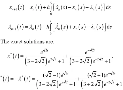
_   _ s

The exact solutions are:

 









2 2

*

2 2 2 2 ,

3 2 2 1 3 2 2 1

t t e e x t e e        

 

 









2 2 * *

2 2 2 2

( 2 1) ( 2 1)

3 2 2 1 3 2 2 1

t t

e e

u t t

e e

   _

   

   

Figure 1, shows the approximate results obtained from the above iteration formulas for n = 2. As shown in fig ure1 when

-1

h  approximations are not so good. T improve the accuracy we have to increase iterations, w

o hereas by changing the auxiliary parameter we can accelerate the convergence and establish good estimations by lower iter o . This shows the flexibility and excel-lence of the PIM. Figure 2 is plot of the error for various iterations. It is clear that accuracy of PIM is higher than VIM.

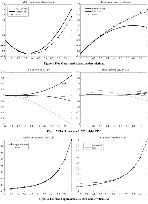
Example 2. Consider the following system: ati ns

 

1





2 2 2

1 1

min 1 d ,

2 2

     

. : 2 , 0 0.9.

0

J x 



x u t

s to x  x t u t x 

 

  

*

u t  k t x t

for k t

 

and its e

According to [4,5],



. In Figure 3, the approximate value xact value are plotted for h 1

of

a . The

exact value

nd optimal value h 0.83

 

k t is

 

5 cosh 5

_



_



sinh 5 1



_



_

osh 5 1 3sinh

k t

t

 

 

Example 3. C ider a 1

5 c 5 1

t t

t

 



ons second-order system as follows:

 

   

 

π 2

2

0

0 0 1

        1 2 0 0 1

min d ,

0 4 2

. : , 0 1, 0 1.

1 0 0

T

J x x u t

s to x x t u t x x

     _{  }  _ _{ } _{ }      





According to Equations (9) and (10), the iteration f mulas are:

or- 

1

0 1 0 0 0

n

t

x t

 

 

0 0

 

1 0

 

d

n n n n

x t h x s x s  s s

[image:3.595.317.534.115.274.2]

[image:4.595.55.539.84.748.2]

Figure 1. Plot of exact and approximation solutions.

Figure 2. Plot of errors, left: VIM, right: PIM.

[image:4.595.56.540.86.293.2]

1063

[image:5.595.59.538.83.295.2]

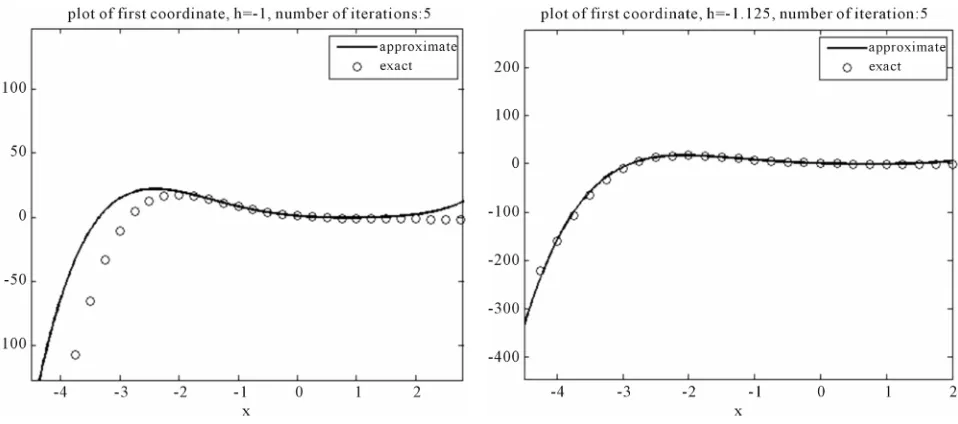
Figure 4. Plot of first coordinate for various h.

[image:5.595.58.541.91.519.2]

Figure 5. Plot of second coordinate for various h.

The exact solutions are:

 

 

 

 

 

1

0

0 0 0 1

d

0 4 0 0

n

t

n n n n

t

t h s x s s s



  



     

  _ _{ } _{  }

   

 





 

























* π π

1 2π

π 2π π π 1

1 cos 1 3 sin

1

cos 3 sin

t

t

x t e e t e

e

e e e t e e t



 _   





    _

t

 

























* π π

2 2π

π 2π π

1 _{1 cos 2 sin}

1

cos 2 sin

t

t

x t e e t e

e

e e e t e t



 _    





     _

 













 









* π π

2π

2π π π

1 _{4 cos 2 2 sin}

1

4 cos 2 2 sin

t

t

u t e e t e t

e

e t e e t



 _    





    _

Figures 4 and 5 show the exact and approximate solu-tions. This problem was solved by VIM in [5] and their presented solutions are only in a small region [1.4, 1.7].

5. Conclusion

and decreases the number of iteration

e interesting for using in the softwars. One idea to esti-mate optimal h mentioned in the paper. In general finding optimal auxiliary parameter h and auxiliary functio

s and this ability will b

n

 

H t used fo

, are open problems. This easy to use method can be r nonlinear systems too.

REFERENCES

[1] L. Ntogramatzidis and A. Ferrante, “On the Solution of the Riccati Differential Equation Arising from t Optimal Control Problem,” Systems & Control Le Vol. 59, No. 2, 2010, pp. 114-121.

doi:10.1016/j.sysconle.2009.12.006

he LQ tters,

[2] P. Williams, “A Gauss-Lobatto Quadrature Met Solving Optimal Control Problems,” ANZIAM Journal Vol. 47, 2006, pp. C101-C115.

[3] M. Yamaguti and S. Ushiki, “Chaos in Numerical Analy sis of Ordinary Differential Equations,” Physica D Nonlinear Phenomena, Vol. 3, No. 3, 1981, pp. 618-626.

doi:10.1016/0167-2789(81)90044-0

hod for , -:

. Chen, “Linear Systems and Optimal Control,” Springer-Verlag, Berlin, Heidelberg, 1989.

8

[4] C. K. Chui and G

doi:10.1007/978-3-642-61312-[5] S. A. Yousefi, M. Dehghan and A. Lotfi, “Finding the Optimal Cont a He’s Variational Iteration Met rnal of Computer

hanics and Engineer-173-4179.

rol of Linear Systems vi hod,” International Jou and Mathematics, 2009.

[6] A. Ghorbani, “Toward a New Analytical Method for Solving Nonlinear Fractional Differential Equations,” Computer Methods in Applied Mec

ing, Vol. 197, No. 49-50, 2008, pp. 4

doi:10.1016/j.cma.2008.04.015

[7] J. H. He, “Variational Iteration Method—A Kind of Non- linear Analytical Technique: Some Examples,”

Interna-lving the Nonlinear tional Journal of Non-Linear Mechanics, Vol. 34, 1999, pp. 699-708.

[8] A. Ghorbani and J. S. Nadjafi, “A Piecewise-Spectral Parametric Iteration Method for So

Chaotic Genesio System,” Mathematical and Computer Modeling, Vol. 54, No. 1-2, 2011, pp. 131-139.