http://www.scirp.org/journal/gep ISSN Online: 2327-4344
ISSN Print: 2327-4336
DOI: 10.4236/gep.2017.513003 Dec. 29, 2017 31 Journal of Geoscience and Environment Protection
Statistical Analysis for Assessing Randomness,
Shift and Trend in Rainfall Time Series under
Climate Variability and Change: Case of Senegal
Didier Maria Ndione
1, Soussou Sambou
1, Moussé Landing Sane
1, Seydou Kane
1,
Issa Leye
1, Seni Tamba
2, Mouhamed Talla Cisse
21Hydraulic and Fluids Mechanics Laboratory (HFML), Department of Physics, Faculty of Sciences and technology, Cheikh Anta
Diop University (UCAD), Dakar, Senegal 2Polytechnic High School of Thies, Thies, Senegal
Abstract
The main purpose of this study is to assess the climate variability and change through statistical processing tools that able to highlight annual and monthly rainfall behavior between 1970 and 2010 in six strategical raingauges located in northern (Saint-Louis, Bakel), central (Dakar, Kaolack), and southern (Zi-guinchor, Tambacounda) part of Senegal. Further, differences in sensitivity of statistical tests are also exhibited by applying several tests rather than a single one to check for one behavior. Dependency of results from statistical tests on studied sequence in time series is also shown comparing results of tests applied on two different periods (1970-2010 and 1960-2010). Therefore, between 1970 and 2010, exploratory data analysis is made to give in a visible manner a first idea on rainfall behavior. Then, Statistical characteristics such as the mean, variance, standard deviation, coefficient of variation, skewness and kurtosis are calculated. Subsequently, statistical tests are applied to all retained time series. Kendall and Spearman rank correlation tests allow verifying whether or not annual rainfall observations are independent. Hubert’s procedures of segmentation, Pettitt, Lee Heghinian and Buishand tests allow checking rainfall homogeneity. Trend is un-dertaken by first employing the annual and seasonal Mann-Kendall trend test, and in case of significance, magnitude of trend is calculated by Sen’s slope es-timator tests. All statistical tests are applied in the period of 1960-2010. Ex-planatory analysis data indicates upwards trends for records in northern and cen-tral and trend free for southern records. Application of multiple tests shows that the Kendall and spearman ranks correlation tests lead to same conclu-sion. The difference in tests sensitivity was shown by outcomes of
homogene-How to cite this paper: Ndione, D.M., Sambou, S., Sane, M.L., Kane, S., Leye, I., Tamba, S. and Cisse, M.T. (2017) Statistical Analysis for Assessing Randomness, Shift and Trend in Rainfall Time Series under Climate Variability and Change: Case of Senegal. Journal of Geoscience and Envi-ronment Protection, 5, 31-53.
https://doi.org/10.4236/gep.2017.513003
Received: October 28, 2017 Accepted: December 26, 2017 Published: December 29, 2017
Copyright © 2017 by authors and Scientific Research Publishing Inc. This work is licensed under the Creative Commons Attribution International License (CC BY 4.0).
http://creativecommons.org/licenses/by/4.0/
DOI: 10.4236/gep.2017.513003 32 Journal of Geoscience and Environment Protection ity tests giving different results either in dates of the shift occurrence or in the significance of an eventual shift. A synthesis analysis of results of tests was car-ried out to conclude about rainfall behaviors. Tests for homogeneity show that southern rainfall is homogeneous, while northern and central ones are not. According to trend test, upwards trends in Northern and central rainfall trend free in southern assumption in exploratory data analysis have been confirmed. The Sen’s slop estimator shows that all retained trend can be assumed to li-near type. The same test over the period 1960-2010 shows independence of ob-servations in all raingauges and exhibits neither trends nor breaks. This seems to show a return to a wet period.
Keywords
Senegal, Rainfall, Time Series, Test, Independence, Homogeneity, Shift, Trend
1. Introduction
Trend and shift detection in observed hydroclimatic records are important themes in hydrological sciences particularly in the scope of natural climate variability and potential climate change [1]. Climate change and climate variability are one of the most important threats facing humanity and the environment. Many scientific studies in hydroclimatic field are oriented towards determining the states, the causes and consequences of climate variability and change [2] [3]. According to these stu-dies, climate change is due to increased greenhouse gas concentrations, while trend and shift in runoff time series data are consequence of climate change effects, land use change (urbanization, clearing, deforestation and others) or change in man-agement practice [4] [5] [6].
The concept of climate change is not simply an assumption: it has been well assessed by many reliable climate models [7]. Shifts in hydrological time series and warming trends detected in several regions throughout the world are climate change indicators. Climate change has repercussions on environment, hydrological data and human economic and social activities [8]. The Tropical North Africa mon-soon has decreased considerably, and depth of many lakes has diminished up to 100 m [9]. In West Africa, shifts in time series of rainfall have been observed: a wet period occurred between 1930 and 1960, a drought from 1970 to 1980 and gradual return of normal rains in the period from 1990 to 2000. Change in pre-cipitation frequency, intensity, duration and consequently on the hydrological cycle has then been notified by many authors [4] [10]. In Senegal, this style of agricultural practice employs 77% of working people and supplies 12.4% of the daily food [11].
Adaptation strategies to climate related consequences require financial means and a good scientific and technical development level. Many approaches can be used to assess climate change.
DOI: 10.4236/gep.2017.513003 33 Journal of Geoscience and Environment Protection detect visually obvious trend; random behavior in hydrological time series by plot-ting data is plotted against time rather than tesplot-ting them. This method allows se-lecting the appropriate hypothesis for statistical tests [12] [13] [14]. Statistic tests are performed to check the assumed time series behavior (randomness, trend and shifts) from exploratory data analysis. This approach has been used as guidance for the purpose of choosing appropriate model distribution to fit non stationary time series; results show that this approach gives in prior a good overview of the adequate model distribution for given observations [15]. The conclusion found on the basis of exploratory data analysis must be verified using statistical tests. The descriptive statistical tools such as mean, variance, and standard deviation, coef-ficient of variation, skewness and kurtosis may provide information regarding rainfall changes and variability [16]-[21].
The independence between observations in rainfall time series is verified us-ing non-parametric tests. The most tests in use for this purpose are the Pearson’s coefficient (r), Spearman’s rho coefficient (
ρ
) or the Kendall’s coefficient (τ ). It has been noticed that the Kendall’s tau can be an alternative to Spearman’s rho for ranked data [22]. So, in some degrees, correlation between observations in Spear-man’s rho and Kendall’s tau tests for independence assessment is associated to presence of trend in time series [23] [24] [25]. Hence, null hypothesis of random-ness H0 is tested against alternative hypothesis H1.DOI: 10.4236/gep.2017.513003 34 Journal of Geoscience and Environment Protection Naivasha, trend, flow rate and local rainfall variability has been studied. Results show a globally homogeneous situation with nevertheless abrupt changes as well as in precipitations than in flows. In addition to this, a net diminishing of about 9.35 × 10⁶ m3 per year of the volume has been noticed [6]. It has been proven that
changes in rainfall characteristics are one of the most relevant signs showing cur-rent climate alterations [31]. As well as many countries in Western and Central Africa, the Senegal faces climate change and climate variability effects.
This study focuses on assessment of annual and monthly rainfall behavior through Senegal. For that, six rain gauges located in the North (Saint-Louis (SL) and Bakel (BK)), the central (Dakar (DK) and Kaolack (KL)) and the south (Zi-guinchor (ZG) and Tambacounda (TC)) of Senegal have been selected. The used rainfall records cover the period from 1960 to 2010. First, the post-1970 rainfall series are analyzed in order to determine the behavior of corresponding states, and this is due to the fact that 1970 characterize the decline of precipitation in Senegal surrounding. In this period (1970-2010), exploratory data analysis in-volving analysis of histograms and moving average curves is made to detect ob-vious randomness, shift or trend in records. Furthermore, statistical characteris-tics such as the mean, the standard deviation, the coefficients skewness and kur-tosis have been estimated. Taking into account the subjectivity of exploratory data analysis approach, statistical tests for randomness (Kendall and Spearman rank correlation tests), shift (Pettitt and Buishand tests; Lee-Heghinian and Hu-bert procedures) and trend (Mann-Kendall and Sen’s tests) are applied to time series. Trend tests are also applied in monthly and seasonal scale. Indeed, appli-cation of multiple tests to check for a same behavior in a time series is done on one hand for exhibiting unlikeness of tests in term of sensitivity and on one oth-er to confirm or to reject the hypothesis to test using conclusion on the basis of majority balance sheet. Then, the same statistical tests (randomness, shift and trend) will be applied to the period from 1960 to 2010 in order to highlight the dependency of results from statistical tests on interested interval of the time se-ries.
2. Materials and Methods
2.1. Data and Study Area
Senegal is located in the most extreme part West Africa between latitudes of 12˚8N - 16˚41N and longitudes of 11˚21 - 17˚32O. Its area is estimated about 196,712 km2. The climate in this country is constituted by two seasons: a rainy season from
DOI: 10.4236/gep.2017.513003 35 Journal of Geoscience and Environment Protection Figure 1. Position of raingauges through the study area.
Table 1. Information on the used raingauges and exploited data.
Station Station ID Location Data (mm) Period of record
Longitude Latitude
Saint-Louis 38004500 −16.05˚ 16.05˚ Annual and monthly rainfall 1970-2010
Bakel 38007200 −12.45˚ 14.90˚ Annual and monthly rainfall 1970-2010
Dakar 38008100 −17.5˚ 14.73˚ Annual and monthly rainfall 1970-2010
Kaolack 38009700 −16.07˚ 14.13˚ Annual and monthly rainfall 1970-2010
Ziguinchor 38013700 −16.27˚ 12.55˚ Annual and monthly rainfall 1970-2010
Tambacounda 38011300 −13.68˚ 13.77˚ Annual and monthly rainfall 1970-2010
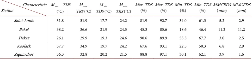
Table 2. Climate characteristics in region surrounding raingauges.
Characteristic
Station max .
M TDS
(˚C)
max . M
TRS (˚C)
min . M
TDS (˚C)
min . M
TRS (˚C)
Max. TDS
(%) Max. TDS (%) Min. TDS (%) Min. TDS (%) MMCEDS (mm) MMCEDS (mm)
Saint-Louis 31.8 31.9 17.7 24.2 81.9 92.7 34.0 61.3 5.2 2.9
Bakel 38.2 36.6 21.9 24.5 45.3 85.6 18.6 46.4 11.2 11.2
Dakar 26.1 29.9 19.3 24.6 90.6 89.9 55.5 67.7 3.0 2.5
Kaolack 37.7 34.9 19.7 24.2 67.6 93.1 22.5 50.3 6.8 2.9
Ziguinchor 36.3 32.8 20.2 21.5 88.8 97.1 30.1 62.1 3.9 1.6
In Table 1, raingauges characteristics, rainfall patterns and period of records are listed. In addition, for each station, mean of maximum temperature during the dry and the rainy season (Mmax TDS and Mmax TRS) is shown in Table 2which
mean of minimum temperature during the dry and the rainy season (Mmin TDS
and Mmin TRS), maximum of the air moisture during the dry and the rainy
[image:5.595.56.540.494.607.2]DOI: 10.4236/gep.2017.513003 36 Journal of Geoscience and Environment Protection cumulative evaporation during the dry and the rainy season (MMCEDS and MMCERS).
2.2. Exploratory Data Analysis and Descriptive Statistic Tools
In this study, the first step in assessment of the rainfall behavior is exploratory data analysis. This is a graphical method in which data are plotted versus time. It allows visually checking out for randomness, shift or trend in time series observing histograms and moving average curves [12] [13]. The exploratory data analysis is a subjective method and is completed in this study by statistical tests. Descriptive statistic tools are used estimating statistic parameters of the time series (mean, standard deviation, coefficient of variation) and the probability distribution (kur-tosis, skewness). The use of above statistical tools allows having an overview on variability of the data through the study area and their dispersion [19]. Indeed, the normal distribution is used as standard base for characterizing probability distribution of the data [19] [32].2.3. Tests for Checking Independency of the Data in a Time Series
The Kendall and the Spearman rank correlation test ([33] [34] [35] [36] [37])are applied in this paper to check for randomness of observations in time series. For both tests, the null hypothesis H0 is the randomness of occurrences andsignifi-cant level is fixed at 5%. We shortly describe the two tests below.
2.3.1. Kendall’s Rank Correlation Test
The Kendall’s rank correlation test is used to test the significance of random be-havior or trend in hydroclimatic time series. It is an efficient tool for verifying linear behavior in time series, and is also referred as τ test. The Kendall’s rank correlation test is based on determining a P number of the subsequent pairs
(
x xi, j)
in the time series satisfying xi<xj(
i< j)
[24] [25] [38]. For a given timeseries X ii
(
=1, 2, 3, 4,,N)
, P is calculated using all(
x xi, j)
combinations, with:1, 2, , 1
i= N− and j= +i 1,,N. The Kendall τ statistic to be tested is as-sumed to be of zero mean with its standard deviation are given by two following equations [24] [25]:
(
4 1)
1P N N
τ =
− −
(1)
( )
(
(
)
)
1 2
2 2 5
9 1
n n n
σ τ = +−
(2) The corresponding standardized statistic Z is given by:
( )
Z τ
σ τ =
(3)
The null hypothesis H0 is accepted when Z belongs to the confident interval:
( )
( )
1 2 , 1 2
Z−α
σ τ
Z−ασ τ
−
DOI: 10.4236/gep.2017.513003 37 Journal of Geoscience and Environment Protection
2.3.2. Spearman’s Rank Correlation Test
The number of observations noticed by N in the time series is first classified in ascending order. Then, the rank of each observation corresponds to its position in the classification is considered [22] [38]. If Rxi and Ryi represent the observations
of xi and yi respectively, the Spearman’s ρ statistic is given by:
(
)
(
)
1 1 1 2 2 1 1 2 2 1 1 i i i i i i i N NN x y
x y N N x y N N x y R R R R N R R R R N N ρ − = − −
∑ ∑
∑
∑
∑
∑
∑
(5)If the number of the observations exceeds 10, the Student t-test can be used rather than the statistic table of Spearman. Then the statistic variable for the test is:
(
)
(
2)
2 1 N t ρ ρ − =
− (6)
For
α
=0.05 , the null hypothesis H0 of randomness is accepted if2.023
t ≤ .
2.4. Tests for Shifts Detection
Observations in time series are assumed to be homogeneous if all data in the times series can be considered as belonging statistically to the same population, that is that they simply follow the same statistical distribution law [24] [39] [40]. In this study, we use Hubert procedure of segmentation of time series, Lee-Heghinian procedure, Pettitt and Buishand [24]. The null hypothesis H0 is the homogeneity
of the time series and the significance level is of
α
=0.05. These tests are brieflydescribed below.
2.4.1. Hubert Procedure of Segmentation
In the Hubert’s process, the time series is divided into consecutive segments m, with m>1 and satisfying the Scheffe’s test [24]. Means of different segments must
be significantly different to the mean of the raw data. The tests in Hubert proce-dure of segmentation, involves the use of the quadratic deviation Dm between row
observations and the means of all m retained segments, is estimated for the sta-tistic test. Let’s consider i kk
(
=1, 2,,m)
the rank of the last observation of akth validate segment in the raw time series
t
X , the spread and the mean of
cor-responding segment shall be respectively:
1
k k k
n = −i i− (7)
1 0 1 1 whith 0 k k i k i i i k
x x i
n = −+
=
∑
=(8)
For a considered series Xt, segmented into m sequences, the quadratic
DOI: 10.4236/gep.2017.513003 38 Journal of Geoscience and Environment Protection 1 m m k k D d =
=
∑
(9)
(
)
1 2 1 k k ik i k
i i
d x x
−
= +
=
∑
−
(10) An acceptable segmentation must verify the Scheffe’s test condition in which
m
D is constrained to be minimal and the mean of the contiguous segments
1
k k
x ≠x+ significantly different.
2.4.2. Procedure of Lee-Heghinian (L-H)
This is a procedure of Bayesian type that is based on an assumption of a single shift in the time series. Variables are supposed in prior independence and uniformly distributed. This model project requires a consideration of following characteristics of the times series: the timing of the shift occurrence noted
τ
s(
1≤ ≤ −τ
s N 1)
,the magnitude of the change in the mean noted δ, the mean of overall data noted by μ and the residual component εi that is a normal and random variable with zero
mean and variance σ2. In this study, the approach used is only based on
post-erior marginal distributions of the shift position in time τs [24] [41]. Then, the
ba-sic mathematical formulation of the Procedure is:
if 1, 2, ,
if 1, ,
i s i i s i x i N
µ ε τ
µ ε δ τ
+ =
= + + = +
(11)
In Equation (11) εi are fluctuations around the mean that are assumed
ran-dom and normal variables with zero mean and unknown variance σ2. The
va-riables µ τ, s and
δ
are respectively the mean, the shift timing and themag-nitude of the change. Considering that the prior probability density of τs is
uni-form, hence, its posterior probability will be:
(
)
( )
( )(
)
1 2
2 2
for 1 1
N s
s s
s s
N
P R N
X N
τ τ τ
τ τ − − ∝ ≤ ≤ − −
(12)
with
( )
(
)
(
)
(
)
2 2 1 1 2 1 ss s s
N
i i N
i i
s N
i N
i
X X X X
R
X X
τ
τ τ τ
τ = = + −
= − + − = −
∑
∑
∑
(13)where: 1 1
N
N i i
X = N
∑
=X (Mean of the raw data); 1 s1s s i i
Xτ = τ
∑
τ=X (Meanbefore date of the shift); s 1 s1
N
N s i i
X −τ = N−τ
∑
= +τ X (Mean after date of theshift).
In cases of unimodal distribution, the shift point is estimated by the mode of above marginal posterior distribution of τs.
2.4.3. Pettitt Test
DOI: 10.4236/gep.2017.513003 39 Journal of Geoscience and Environment Protection into two subsequences x tt
(
=1, 2, 3,,τ
s)
and x tt(
= +τ
s 1,N)
. Thus,probabil-ity distribution functions F X1
( )
and F2( )
X can be associated to the twosub-sequences respectively. In practice, the null hypothesis H0 is F X1
( )
=F2( )
X andthe alternative hypothesis H1 is F X1
( )
≠F2( )
X [24]. This method involves alsoa comparison of the observations so that:
(
)
(
(
)
)
(
)
,
1 if 0
sgn 0 if 0
1 if 0
i j
i j i j i j
i j
x x
D x x x x
x x
− >
= − − =
− − <
(14)
Then for the implementation of the statistic variable to use for the test, a basic variable Uτs,N is defined as:
, , 1 1 , 1 s s s N
N i j s
t t
U D N
τ τ
τ
τ
= = +=
∑ ∑
≤ ≤ (15)Using the theory on statistic ranks, another KN variable is derived from
,
sN
Uτ . This new variable is defined as [42]:
(
)
,
max 1, 2, , 1
s
N N s
K = Uτ
τ
= N− (16)For the test, a probability of exceedance is fixed for a threshold value k given by the formula:
(
N)
6 exp(
3(
622)
)
k P K k
N N
− > ≅
+ (17)
The null hypothesis, H0 is rejected if the probability of exceedance given in
equation 17 is less than the significant level α for a one-sided statistic test. Hence, the shift in the time series is observed at the time τ =s t corresponding to the
date of the occurrence of the retained KN.
2.4.4. Buishand’s U Statistic and Bois’s Ellipse
The Buishand’s U statistic is inferred from a formulation of shift point detecting in Gardne, 1969 [43]. This test is performed under assumption of a single shift in mean of the time series with unknown variance [24] [39]. The method requires normal distribution of the data, then, under the above single shift assumption, the time series is modeled as follow:
for 0, for 1, i s i i s i x i N µ τ
µ δ τ
+ ∈
= + + ∈ +
(18)
where i are fluctuations around the mean that are assumed random and
nor-mal variables with zero mean and unknown variance σ2. In Equation (18), ,
µ τ
andδ
are the same that of define in the Lee-Heghinian test (Equation (11)). The statistic test in this approach is performed on the basis of cumulative deviation from the mean given by:(
)
01
with 0; 1, ,
k
k i
i
S x x S k N
=
DOI: 10.4236/gep.2017.513003 40 Journal of Geoscience and Environment Protection
k
S is assumed to be normally distributed with zero mean. The Buishand’s U is
then defined using Sk and replacing the unknown variance by that of the raw
data noticed by 2
x
D (Equation (21)). The U is expressed as:
(
)
(
)
1 1(
)
21 1
N
k x
k
U N N S D
− −
=
= +
∑
(20)
(
)
22 1
1
N
x i i
D =N−
∑
= X −X (21)The test is made using an estimate of above unknown variance expressed in Equa-tion (18). Estimate of the unknown is carried out to define the confident limit and is given by:
(
)(
)
12 2
ˆ k N k N 1 D kx, 0, ,N
σ
= − − − = (22)
The confidence interval that should contain the Buishand’s U if the null hypo-thesis is accepted is given by an ellipse of control. The function defining the el-lipse is implemented employing the estimate 2
ˆ
σ [39]:
( )
1 2
1 x
k N k
U α N D
− −
± −
(23)
For a given significant level α , the null hypothesis H0 is rejected if the
Buishand’s U goes out of the confidence area surrounded by the ellipse of con-trol.
2.5. Tests for Trend Detection and Moving Average Curve
Trend tests are used in time series analysis to determine the direction of the data overall evolution in time. A declared trend indicates increasing or decreasing evo-lution in measured observations. It is important to highlight the fact that trend free in time series doesn’t mean a case of equality in records. These tests are used in this study to supplement the graphical approach (Exploratory Data Analysis) in which histograms moving average curves was exploited. The moving average method fil-ters the obvious irregularities in the time series [25]. The annual Mann-Kendall test is called upon for trend assessment in the annual rainfall depth. Then the Sen’s slope estimator is used to estimate the linearity of the trend and its magnitude. The seasonal and monthly tests of Mann-Kendall are also carried out to complete the rainfall trend investigation.
2.5.1. Linear Moving Average Filtering Method
The moving average curve (MA) aims to filter short-term effects in time series. This approach of trend assessment involves weighting of a limited range of (2k + 1) values of the raw time series Xt to transform it seems to be the most
com-monly used type [25]. Then, a new transformed series Yt is obtained with
sub-stantial reduction of original short-term fluctuations:
(
)
11
2 1
k
t t j
j k
Y X
k − =− + =
DOI: 10.4236/gep.2017.513003 41 Journal of Geoscience and Environment Protection
2.5.2. The Man-Kendall Test
The Mann-Kendall (M-K) test is use in time series analysis to detect a trend and its direction without specifying whether the trend is linear or not [44]. The me-thod is based on one statistic S. The statistic S is determined by result from a comparison between each pair of observations
(
x xi, j)
with i< j, to find out ,i j
x >x , xi<xj or xi=xj. A score of 1, −1 or 0 is associated for each case
de-pending on the sign of the difference between pairs. Then explicitly, the M-K S statistic to be tested defined as [25] [45] [46] [47] [48] [49]:
(
)
1 1 1 sgn N N j ii j i
S x x
−
= = +
=
∑ ∑
−(25)
With
(
)
(
)
(
)
(
)
(
)
(
)
sgn 1 if 0
sgn 0 if 0
sgn 1 if 0
j i j i
j i j i
j i j i
x x x x x x x x x x x x
− = − >
− = − =
− = − − <
(26)
A negative value of S indicates falling trend, while a positive value of the S in-dicates rising trend. Then, the S is assumed to be independent and normally dis-tributed with zero mean and variance given by:
( )
(
1 2)(
5)
Var
18
N N N
S = − + (27)
Hence, the Z normal standard distribution of the M-K S can be defined as:
(
)
( )
(
)
( )
1 if 0 var0 if 0
1 if 0 var S Z S S Z S S Z S S − = > = = −
= <
(28)
The null hypothesis H0 is accepted if the P value exceeds 0.05. 2.5.3. Sen’s Slope Estimator
In this method, for each pair of observations
(
x xi, j)
an associated slope canna-turally be given as:
, j i i j x x S j i − =
− (29)
where xj and xi are observations at time j and i
(
i< j)
respectively. In asam-ple of size N, the number of slopes one can obtained is given by n=N N
(
−1 2)
.The Sen’s slope estimator is given by the median slope estimated after ranking the n slopes in an increasing order. If n is odd number, the median slop (MS) is given by the formula: Q( )n+1 2, while, if it is even by
{
Qn2+Q(n+2 2) }
2. Thenull hypothesis is accepted if the estimated median slope is within the range of
(
n Cα)
2 and(
n Cα)
2 − +
, where 1
( )
2 Var
Cα Z α S
−
Equa-DOI: 10.4236/gep.2017.513003 42 Journal of Geoscience and Environment Protection tion (27), in the assumption of no tied value in the time series [35] [36] [47] [50] [51].
[image:12.595.84.542.267.712.2]3. Results and Discussion
3.1. Exploratory Analysis of Data
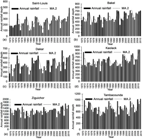
Figure 2 presents the temporal variation of annual rainfall for all rain gauges by the mean of histograms and moving average curves of order 2 (MA.2). In explo-ratory analysis, shifts are not obvious, while random behavior for Ziguinchor (Figure 2(e)) and Tambacounda (Figure 2(f)) can be assumed. Furthermore, up-wards trends seam to appear for Saint-Louis (Figure 2(a)), Dakar (Figure 2(c)), Bakel (Figure 2(b)) and Kaolack (Figure 2(d)) raingauges, while Tambacounda and Zi-guinchor seem to be trend free.
DOI: 10.4236/gep.2017.513003 43 Journal of Geoscience and Environment Protection
3.2. Statistical Characteristics of Annual Rainfall
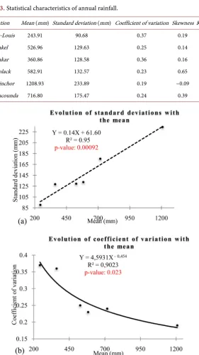
[image:13.595.231.513.201.703.2]The statistical characteristics of the annual rainfall are given in Table 3. The anal-ysis of the means (Figure 3(a)) and the standard deviation over the period of 1970-2010 shows that the rainfall decreases from South to North and from East to West. The coefficient of variation decreases as the rainfall increases in magni-tude (Figure 3(b)). So, the less the rainfall the unsteady they are. Distributions of annual rainfall are positively skewed for all rain gauges except that at Ziguinchor and are all platykurtic except that at Kaolack.
Table 3. Statistical characteristics of annual rainfall.
Station Mean (mm) Standard deviation (mm) Coefficient of variation Skewness Kurtosis
Saint-Louis 243.91 90.68 0.37 0.19 −0.09
Bakel 526.96 129.63 0.25 0.14 −0.75
Dakar 360.86 128.58 0.36 0.16 −0.68
Kaolack 582.91 132.57 0.23 0.65 0.32
Ziguinchor 1208.93 233.89 0.19 −0.09 −0.47
Tambacounda 716.80 175.47 0.24 0.39 −0.74
DOI: 10.4236/gep.2017.513003 44 Journal of Geoscience and Environment Protection
3.3. Synthesis of Tests for Independence
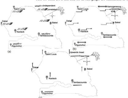
Results of independency test for all times series using Kendall tau and Spearman rho testsare presented inTable 4. It has been noticed that both above tests lead to same results: the null hypothesis of independence (I) is rejected for all rain gauges except for Ziguinchor and Tambacounda. For Saint-Louis, Bakel, Dakar and Kaolack, observations in time series are correlated (C). A special view of the results is given in Figure 4(a).
3.4. Synthesis of Tests for Homogeneity
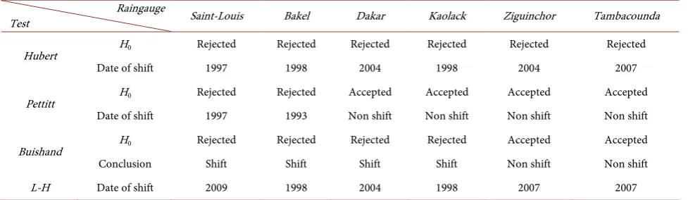
[image:14.595.56.545.567.709.2]The results of all homogeneity tests for annual rainfall between 1970 and 2010 are presented in Table 5. For raingauges at Saint-Louis and Bakel, the null hy-pothesis of homogeneity of rainfall time series is rejected for all tests. For Dakar and Kaolack, null hypothesis is rejected by three of the four tests, while for Zi-guinchor and Tambacounda null hypothesis is rejected by two among the four tests. So, we finally consider that a rainfall time series is non-homogeneous when null hypothesis is rejected by at least three tests among the applied four. This is the case of Saint-Louis, Bakel, Dakar and Kaolack where rainfall time series are
Table 4. Results of tests for independence.
Raingauge
Test Saint-Louis Bakel Dakar Kaolack Ziguinchor Tambacounda
Kendall
Kendall’s τ 0.30 0.33 0.24 0.22 0.19 0.10
Z Statistic 2.78 3.10 2.18 2.10 1.73 0.94
H0 Rejected Rejected Rejected Rejected Accepted Accepted
Conclusion Correlated Correlated Correlated Correlated Independent Independent
Spearman Spearman’s ρ −0.436 −0.438 −0.323 −0.321 −0.239 −1.151
Z Statistic −3.027 −3.042 −2.135 −2.119 −1.540 −0.953
Spearman Conclusion H0 Rejected Rejected Rejected Rejected Accepted Accepted
Correlated Correlated Correlated Correlated Independent Independent
H0: Null hypothesis.
Table 5. Results of tests for homogeneity of rainfall time series from 1970 and 2010.
Raingauge
Test Saint-Louis Bakel Dakar Kaolack Ziguinchor Tambacounda
Hubert H0 Rejected Rejected Rejected Rejected Rejected Rejected
Date of shift 1997 1998 2004 1998 2004 2007
Pettitt H0 Rejected Rejected Accepted Accepted Accepted Accepted
Date of shift 1997 1993 Non shift Non shift Non shift Non shift
Buishand H0 Rejected Rejected Rejected Rejected Accepted Accepted
Conclusion Shift Shift Shift Shift Non shift Non shift
L-H Date of shift 2009 1998 2004 1998 2007 2007
DOI: 10.4236/gep.2017.513003 45 Journal of Geoscience and Environment Protection shifted. For Ziguinchor and Tambacounda, rainfall time series are assumed to be homogeneous. When H0 is rejected, the dates of shift occurrence often vary from
a raingauge to another and also from a test to another. So, we retain as date of shift occurrence in time series, the one indicated by the maximum of tests. Thus, shift occurred at 1997 at Saint-Louis, 1998 at Bakel, and 2004 at Dakar. Zones with and without shifts in rainfall time series through the study area are shown in Figure 4(b).
3.5. Synthesis of Results from Trend Assessment: M-K Test and
Sen’s Slope Estimator
[image:15.595.90.509.231.551.2]Tests for trend (M-K and Sen) for all rain gauges are summarized in Table 6.
Figure 4. Results of tests for independency, shift and trend in the study area from 1970 to 2010.
Table 6. Results of trend tests for rainfall series from 1970 to 2010.
Raingauge
Test Saint. Louis Bakel Dakar Kaolack Ziguinchor Tambacounda
M-K
Mann-Kendall Statistic (M-KS) 2.77 3.74 2.17 2.07 1.92 1.93
H0 Rejected Rejected Rejected Rejected Accepted Accepted
conclusion UT UT UT UT TF TF
Sen’s
Median Slope (MS) 3.21 4.71 4.27 7.35 6.48 2.64
H0 Accepted Accepted Accepted Accepted Accepted Accepted
conclusion NLT NLT NLT NLT NLT NLT
[image:15.595.57.545.603.711.2]DOI: 10.4236/gep.2017.513003 46 Journal of Geoscience and Environment Protection The M-K test is first applied to look for trend significance. Where trend exists, Sen’s slope estimator is used to verify whether it can be considered as of a linear type, then its magnitude. The M-K test detects upwards trend (UT) for rainfall at Saint-Louis, Bakel, Dakar and Kaolack. According to the Sen’s slope estimator, existing trends are of nonlinear type (NLT). In the study area, reparation in space of studied rainfall time series with and without trend are shown in Figure 4(c).
3.6. Results of Tests for Trend at Monthly and Seasonal Scale
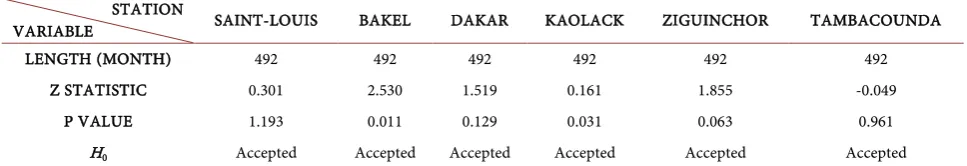
The seasonal and monthly M-K tests are applied from 1970 to 210. Table 7 presents the results of the seasonal M-K test, while in Table 8 are presented results in monthly scale. The seasonal M-K test accepts null hypothesis of no trend for all raingauges and for all seasonal time series except the months of June and September for the raingauge at Kaolack and the month of September for the raingauge at Ziguinchor. At monthly scale no trend has been detected by the M-K tests, although trends have been detected at annual scale.3.7. Relativity of Results from Statistical Tests: Dependency of
Statistical Tests Issues to Period of Study
In this part of the study, we try to know how the period of study impacts the re-sults of the test. We consider two periods of study: 1960-2010 and 1970-2010. The same tests for independency, homogeneity and trend are applied on the two pe-riods and for all raingauges. In this section, indices of (+) is used to define accep-tation of the null hypothesis and (−) for its rejection.
3.7.1. Dependency of Results Independency Tests Issues to Period of Study
[image:16.595.55.543.500.596.2]We compare in Table 9 the results of tests for independence for the two periods
Table 7. Results of the M-K at seasonal scale between 1970 and 2010.
MONTH OBSERVATION STATISTIC Z STATISTIC P VALUE NULLE HYPOTHESIS
STATION OF KAOLACK
JUN 41 222 2.493 0.012 Rejected
SEPTEMBER 41 194 2.179 0.029 Rejected
STATION OF ZIGUINCHOR
SEPTEMBER 41 183 2.055 0.040 Rejected
Table 8. Results of the M-K at monthly scale between 1970 and 2010.
STATION
VARIABLE SAINT-LOUIS BAKEL DAKAR KAOLACK ZIGUINCHOR TAMBACOUNDA
LENGTH (MONTH) 492 492 492 492 492 492
Z STATISTIC 0.301 2.530 1.519 0.161 1.855 -0.049
P VALUE 1.193 0.011 0.129 0.031 0.063 0.961
H0 Accepted Accepted Accepted Accepted Accepted Accepted
[image:16.595.56.540.627.710.2]DOI: 10.4236/gep.2017.513003 47 Journal of Geoscience and Environment Protection Table 9. Results of independence tests for the two periods in comparison.
PERIOD 1960-2010 1970-2010
STATION
TEST SL BK DK KL ZG TB SL BK DK KL ZG TB
KENDALL RANK TEST H0 + + + + + + − − − − + +
conclusion C C C C C C C C C C I I
SPEARMAN RANK TEST H0 + + + + + + − − − − + +
conclusion I I I I I I C C C C I I
C: correlated; I: independent; H0: Null hypothesis; +: H0 accepted; −: H0 rejected.
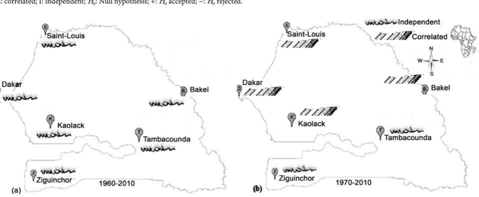
Figure 5. Effect of the period on tests for independence.
of study. The period of study does not impact the results of the test for Ziguin-chor and Tambacounda raingauges. We note that annual rainfall is more im-portant for these stations. Figure 5(a) & Figure 5(b) shows locations where outcomes of randomness tests were impacted or not by the variation in time se-ries sequence.
3.7.2. Dependency of Homogeneity Tests Issues to Period of Study
[image:17.595.61.541.192.389.2]DOI: 10.4236/gep.2017.513003 48 Journal of Geoscience and Environment Protection Table 10. Results of homogeneity tests for the two periods in comparison.
PERIOD 1960-2010 1970-2010
STATION
TEST SL BK DK KL ZG TB SL BK DK KL ZG TB
HUBERT H0 − + − − + − − − − − − +
Conclusion 1969 H 1969 1971 H 1966 1997 1998 2004 1998 2004 2007
PETTITT H0 + + + + − − − + + + + +
Conclusion H H H H H 1975 1997 1993 H H H H
BUISHAND H0 + + + + + + + + + + + +
Conclusion H H H H H S S S S S H H
L-H Conclusion 1969 1998 1969 1967 1960 1966 2009 1998 2004 1998 2007 2007
h: Homogeneous; s: shift; L-H: Lee-Heghinian; H0: Null hypothesis; +: H0 accepted; −: H0 rejected.
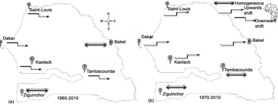
Figure 6. Effect of the period on tests for homogeneity.
3.7.3. Dependency of Trend Tests Issues to Period of Study
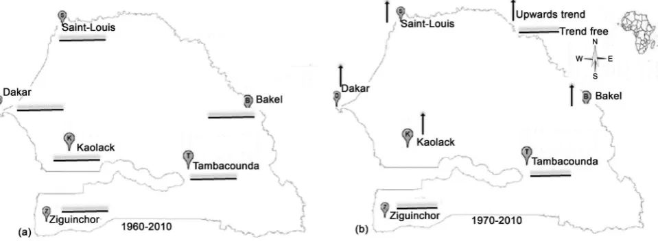
Results of tests for trend between the two periods are compared in Table 11. The application of the tests for trend between 1960 and 2010 does not detect any trend. For the period 1970 to 2010, we note upward trends (UT) in Central and North-ern Senegal, while annual rainfall in SouthNorth-ern (Tambacounda and Ziguinchor) are trend free (TF). The period of study doesn’t impact Ziguinchor and Tamba-counda raingauges. For the other stations, upwards trend during the second pe-riod seems to indicate a come back to a rainy pepe-riod. Locations where outcomes of trend tests were impacted or not by the variation in time series sequence are indicated in Figure 7(a) & Figure 7(b).
4. Conclusion
[image:18.595.59.540.273.455.2]DOI: 10.4236/gep.2017.513003 49 Journal of Geoscience and Environment Protection Table 11. Results of trend tests for the two periods in comparison.
Period 1960-2010 1970-2010
Station
Tests SL BK DK KL ZG TB SL BK DK KL ZG TB
M-K
H0 + + + + + + − − − − + +
M-KZS 0.32 −0.50 1.04 0.28 −0.66 −0.82 2.77 3.74 2.17 2.07 1.92 1.93
Conclusion TF TF TF TF TF TF UT UT UT UT TF TF
Sen’s
H0 + + + + + + + + + + + +
MS 0.31 1.44 −1.32 −1.42 −3.06 −3.06 3.21 4.71 4.27 7.35 6.48 2.64
Conclusion NLT NLT NLT NLT NLT NLT NLT NLT NLT NLT NLT NLT
TF: Trend free; UT: Upwards trend; NLT: Nonlinear trend; H0: Null hypothesis; M-KZS: The M-K Z Statistic; MS: Median Slope; H0: Null Hypothesis; +: H0
Accepted; −: H0 Rejected.
Figure 7. Effect of the time series sequences on tests for trend.
[image:19.595.60.540.265.441.2]DOI: 10.4236/gep.2017.513003 50 Journal of Geoscience and Environment Protection to this analysis, the high magnitude of rainfall depth from 1960 to 1970 included in the second involved period impacted the results. They have disturbed retained shift dates, inhibited confirmed upward rainfall trends and non-randomness of observations from the study focused on the period of 1970-2010. Hence, ran-domness tests (Kendall and Spearman ranks), if used as trend test lead to same results as the M-K one.
References
[1] Ishak, E. and Rahman, A. (2015) Detection of Changes in Flood Data in Victoria, Australia from 1975 to 2011. Hydrology Research, 46, 663-676.
https://doi.org/10.2166/nh.2014.064
[2] Yao, A.B., Goula, B.T.A., Kouadio, Z.A., Kouakou, K.E., Kane, A. and Sambou, S. (2012) Analyse de la variabilité climatique et quantification des ressources en eau en zone tropicale humide: Cas du bassin versant de la Lobo au centre-ouest de la côte d’ivoire. Revue Ivoirienne des Sciences et Technologie, 19, 136-157.
[3] Joanne, I. and Turton, S. (2014) Expansion of the Tropics. Essay, 5, 435-447. [4] Notaro, V., Liuzzo, L., Freni, G. and La Loggia, G. (2015) Uncertainty Analysis in
the Evaluation of Extreme Rainfall Trends and Its Implications on Urban Drainage System Design. Water, 7, 6931-6945.https://doi.org/10.3390/w7126667
[5] Foltz, G.R. and McPhaden, M.J. (2008) Trends in Saharan Dust and Tropical Atlantic Climate during 1980-2006. Geophysical Research Letters, 35, 1-5.
https://doi.org/10.1029/2008GL035042
[6] Odongo, V.O., Van der Tol, C., Van Oel, P.R., Meins, F.M., Becht, R., Onyando, J. and Su, Z. (2015) Characterisation of Hydroclimatological Trends and Variability in the Lake Naivasha Basin, Kenya. Hydrological Processes, 29, 3276-3293.
https://doi.org/10.1002/hyp.10443
[7] IPCC (2007) Climate Change 2007: The Physical Science Basis. In: Solomon, S., Qin, D., Manning, M., Chen, Z., Marquis, M., Averyt, K.B., Tignor, M. and Miller, H.L., Eds., Contribution of Working Group I to the 4th Assessment Report of the Intergovernmental Panel on Climate Change, Cambridge University Press, Cambridge and New York, 996 p.
[8] Seidel, D.J., Fu, Q., Randel, W.J. and Reichler, T.J. (2008) Widening of the Tropical Belt in a Changing Climate. Nature Geoscience, 1, 21-24.
[9] Kutzbach, J.E. and Street-Perrott, F.A. (1985) Milankovitch Forcing of Fluctuations in the Level of Tropical Lakes from 18 to 0 kyr BP. Nature, 317, 130-134.
https://doi.org/10.1038/317130a0
[10] Dieppois, B., Diedhiou, A., Durand, A., Fournier, M., Massei, N., Sebag, D., Xue, Y. and Fontaine, B. (2013) Quasi-Decadal Signals of Sahel Rainfall and West African Monsoon since the Mid-Twentieth Century. Atmospheres, 118, 1-13.
https://doi.org/10.1002/2013JD019681
[11] USGS, USAID (2012) Famine Earl Warning Systems Network—Informing Climate Change Adaptation Series. A Climate Trend Analysis of Senegal. Rolla Publishing Service Center. https://pubs.usgs.gov/fs/2012/3123/FS12-3123.pdf
[12] Costa, A.C., Durao, R., Soares, A. and Pereira, M.J. (2008) A Geostatistical Exploratory Analysis of Precipitation Extremes in Southern Portugal. REVSTAT—Statistical Journal, 6, 21-32.
DOI: 10.4236/gep.2017.513003 51 Journal of Geoscience and Environment Protection Hydrological Data. World Climate Program Data and Monitoring. WMO/TD-No. 1013.
[14] Hosseini Le, N.D. and Zidek, J.V. (2009) An Analysis of Alberta’s Climate. Part I: Non-Homogenized Data. University of British Columbia. Department of Statistics Technical Report 245.
[15] Serinaldi, F. and Kilsby, C.G. (2015) Stationarity Is Undead: Uncertainty Dominates the Distribution of Extremes. Advances in Water Resources, 77, 17-36.
https://doi.org/10.1016/j.advwatres.2014.12.013
[16] Bai, J. and Ng, S. (2005) Tests for Skewness, Kurtosis, and Normality for Time Series Data. Journal of Business & Economic Statistics, 23, 49-60.
https://doi.org/10.1198/073500104000000271
[17] Sen, A.K. and Niedzielski, T. (2010) Statistical Characteristics of Riverflow Variabilityin the Odra River Basin, Southwestern Poland. Original Research, 19, 387-397. [18] Mzezewa, J., Misi, T. and Van Rensburg, L.D. (2010) Characterization of Rainfall at
a Semi-Arid Ecotope in the Limpopo Province (South Africa) and Its Implications for Sustainable Crop Production. Water SA, 36, 19-26.
https://doi.org/10.4314/wsa.v36i1.50903
[19] Yusof, F. and Hui-Mean, F. (2012) Use of Statistical Distribution for Drought Analysis. Applied Mathematical Sciences, 6, 1031-1051.
[20] Baldassarre, G.D., Castellarin, A. and Brath, A. (2006) Relationships between Statistics of Rainfall Extremes and Meanannual Precipitation: An Application for Design-Storm Estimation Innorthern Central Italy. Hydrology and Earth System Sciences, 10, 589-601.https://doi.org/10.5194/hess-10-589-2006
[21] Lanzante, J.R. (1996) Resistant, Robust and Non-Parametric Techniques for the Analysis of Climate Data: Theory and Examples, Including Applications to Historical Radiosonde Station Data. International Journal of Climatology, 16, 1197-1226.
https://doi.org/10.1002/(SICI)1097-0088(199611)16:11<1197::AID-JOC89>3.0.CO;2 -L
[22] Hauke, J. and Kossowski, T. (2011) Comparison of Values of Pearson’s and Spearman’s Correlation Coefficients on the Same Sets of Data. QuaestionesGeographicae, 30, 87-93.
[23] Wang, W., Chen, Y., Becker, S. and Liu, B. (2015) Linear Trend Detection in Serially Dependent Hydrometeorological Data Based on a Variance Correction Spearman Rho Method. Water, 7, 7045-7065.https://doi.org/10.3390/w7126673
[24] Lubes-Niel, H., Masson, J.M., Paturel, J. and Servat, E. (1998) Climatique Variability and Statistics. A Simulation Approach for Estimating Power and Robustness of Tests of Stationarity. Journal of Water Science, 11, 383-408.
[25] Kottegoda, N.T. (1980) Stochastic Water Resources Technology. The Mac Millan Press Ltd., Department of Civil Engineering, University of Birmingham.
https://doi.org/10.1007/978-1-349-03467-3
[26] Soro, T.D., Soro, N., Oga, Y.M.S., Lasm, T., Soro, G., Ahoussi, K.E. and Biemi, J. (2011) La variabilité climatique et son impact sur les ressources en eau dans le degré carré de Grand-Lahou (Sud-Ouest de la Côte d’Ivoire). Physio-géo, 5, 55-73.
https://doi.org/10.4000/physio-geo.1581
[27] Paturel, J.E., Servat, E. and Kouame, B. (1997) Manifestations d’une variabilité hydrologique en Afrique de l’Ouest et Centrale. IAHS Publ, Vol. 240, 22-30. [28] Sebbar, A., Badri, W., Fougrach, H., Hsaine, M. and Saloui, A. (2011) Etude de la
DOI: 10.4236/gep.2017.513003 52 Journal of Geoscience and Environment Protection 22, 139-148.
[29] Bolakonga, I. and Ozer, P. (2007) Analyse de la variabilité des précipitations sahéliennes et évaluation des impacts sur l’environnement de quelques localités nigériennes et maliennes. Annales de l’Institut Facultaire des Sciences Agronomiques de Yangambi, 1, 48-61.
[30] Qin, N., Chen, X., Fu, G., Zhai, J. and Xue, X. (2010) Precipitation and Temperature Trends for the Southwest China: 1960-2007. Hydrological Processes, 24, 3733-3744.
https://doi.org/10.1002/hyp.7792
[31] Arnone, E., Pumo, D., Viola, F., Noto, L.V. and La Loggia, G. (2013) Rainfall Statistics Changes in Sicily. Hydrology and Earth System Sciences, 17, 2449-2458.
https://doi.org/10.5194/hess-17-2449-2013
[32] DeCarlo, L.T. (1997) On the Meaning and Use of Kurtosis. Psychological Methods, 3, 292-307.https://doi.org/10.1037/1082-989X.2.3.292
[33] Machiwal, D. and Jha, M.K. (2006) Time Series Analysis of Hydrologic Data for Water Resources Planning and Management: A Review. Journal of Hydrology and Hydromechanics, 3, 237-257.
[34] WMO (1966) Climatic Change, by a Working Group of the Commission. TP 100, Tech. Note, 79, 78.
[35] Kahya, E. and Kalay, S. (2004) Trend Analysis of Streamflow in Turkey. Journal of Hydrology, 289, 128-144.https://doi.org/10.1016/j.jhydrol.2003.11.006
[36] Fathian, F., Morid, S. and Kahya, E. (2014) Identification of Trends in Hydrological and Climatic Variables in Urmia Lake Basin, Iran. Theoretical and Applied Climatology, 119, 443-464.https://doi.org/10.1007/s00704-014-1120-4
[37] Hamed, K.H. (2016) The Distribution of Spearman’s Rho Trend Statistic for Persistent Hydrologic Data. Hydrological Sciences Journal, 61, 214-223.
https://doi.org/10.1080/02626667.2014.968573
[38] Zhang, S. and Lu, X.X. (2007) Long Term Water and Sediment Change Detection in a Small Mountainous Tributary of the Lower Pearl River. Hydrological Science, 6, 97-108.
[39] Buishand, T.A. (1984) Test for Detecting a Shift in the Mean of Hydrological Time Series. Journal of Hydrology, 73, 51-69.
https://doi.org/10.1016/0022-1694(84)90032-5
[40] Ondo, J.C. and Ouarda, T. (1997) Revue bibliographique des tests d’homogénéités. Institut national de la recherche cientifique. Eau 2800, rue Einstein, CP. 7500 Saint-Foy C1V4C7. Rapport de recherche n R-500, Québec.
[41] Baman, A.D., Bado, B.V., Sambou, S. and Gaye, C.B. (2013) Anti-Salt Dam as a Means of Recovering Lowland Degraded by Sea Water: The Case of Lowland Ndour Ndour, Senegal. American Journal of Environmental Protection, 2, 79-84.
[42] Pettitt, A.N. (1979) A Non-Parametric Approach to the Change-Point Problem. Journal of Applied Statistics, 28, 126-135.https://doi.org/10.2307/2346729
[43] Gardne, L.A. (1969) On Detecting Changes in the Mean of Normal Variâtes. The Annals of Mathematical Statistics, 40, 116-126.
https://doi.org/10.1214/aoms/1177697808
[44] Khaliq, M.N., Ouarda, T.B.M.J., Gachon, P., Sushama, L. and St-Hilaire, A. (2009) Identification of Hydrological Trends in the Presence of Serial and Cross Correlations: A Review of Selected Methods and Their Application to Annual Flow Regimes of Canadian Rivers. Journal of Hydrology, 368, 117-130.
DOI: 10.4236/gep.2017.513003 53 Journal of Geoscience and Environment Protection [45] Önöz, B. and Bayazit, M. (2003) The Power of Statistic Tests for Trend Detection.
Turkish Journal of Engineering and Environmental Sciences, 27, 247-251. [46] Keredin, T.S., Annissa, M., Surendra, B. and Solomon, A. (2009) Long Years
Com-parative Climate Change Trend Analysis in Terms of Temperature, Coastal Andhra Pradesh, India. National Monthly Refereed Journal of Research in Science and Technology, 2, 1-13.
[47] Tesemma, Z.K., Mohamed, A.Y. and Steenhui, S. (2010) Trend in Rainfall and Runoff in the Blue Nil Basin. Hydrological Processes, 24, 3747-3758.
https://doi.org/10.1002/hyp.7893
[48] Luo, Y., Fu, S., Liu, J., Wang, G. and Zhou, G. (2008) Trend of Precipitation Beijiang River Basin, Guangdong Province, China. Hydrological Processes, 22, 2377-2836.https://doi.org/10.1002/hyp.6801
[49] Yue, S. and Pilon, P. (2004) A Comparison of the Power of the Test, Mann-Kendall and Bootstrap Tests for Trend Detection. Journal des Sciences Hydrologiques, 49, 21-37.https://doi.org/10.1623/hysj.49.1.21.53996
[50] Salmi, T., Maatta, A., Anttila, P., Ruoho-Airola, T. and Amnel, T. (2002) Detecting Trends of Annual Values of Atmospheric Pollutants by the Mann-Kendall Test and Sen’s Slope Estimates—The Excel Template Application Makesens. Finnish Meteorological Institute, Vol. 31, 1-35.