Bayesian Student Modelling and Decision Theoretic Selection of Tutorial Actions in Intelligent Tutoring Systems

(1)

Decision-Theoretic Selection of Tutorial

Actions in Intelligent Tutoring Systems

A THESIS

SUBMITTED IN PARTIAL FULFILMENT

OF THE REQUIREMENTS FOR THE DEGREE OF

DOCTOR OF PHILOSOPHY IN COMPUTER SCIENCE IN THE

UNIVERSITY OF CANTERBURY by

Michael John Mayo

(2)

(3)

(4)

i

Acknowledgements

First of all, I want to thank my loving and ever patient wife Nhung. Without her support, none of this would have been possible.

I would also like to thank my supervisor, Tanja Mitrovic, for her advice and guidance over the years. It was invaluable. Thanks also to both Tanja and Jane McKenzie for reading drafts of this thesis.

During my time as a student, I wrote a number of papers for publication based on the research and ideas presented here. I would like to thank the anonymous reviewers for their helpful comments and criticism.

Financial assistance was provided from the Department of Computer Science. For that, I am highly grateful.

Kurt Hausler was employed to do some of the programming for the SQL-Tutor evaluation study described in Chapter 4. Thanks, Kurt.

Microsoft provided the Bayesian networks API used in the implementation of CAPIT.

Finally, thanks to the numerous participants of the various evaluation studies. These include the numerous undergraduate computer science students who used my version of SQL-Tutor during 1999, and the staff and students of Westburn and Ilam School in Christchurch, New Zealand, who used CAPIT in April and June 2000.

MICHAEL MAYO

(5)

(6)

iii

Abstract

This thesis proposes, demonstrates, and evaluates, the concept of the normative Intelligent Tutoring System (ITS). Normative theories are ideal, optimal theories of rational behaviour. Two normative theories suitable for reasoning under conditions of uncertainty are Bayesian probability theory, which allows one to update one’s beliefs about the world given previous beliefs and new observations, and decision theory, which shows how to fuse one’s preferences with one’s beliefs in order to rationally decide how to behave. A normative ITS is a tutoring system in which beliefs about the student (the student model) are represented with a Bayesian network, and teaching actions are selected using decision-theoretic principles. The main advantage of a normative ITS is that the normative theories provide an optimal framework for implementing learning theories. In other words, the particular learning theory underlying the ITS is guaranteed to be optimally applied to the student if it is defined as a set of normative representations (probability distributions and utility functions). In contrast, the more traditional type of ITS with an ad-hoc implementation of a learning theory is not guaranteed to be optimal.

A general methodology for building normative ITSs is proposed and demonstrated. The methodology advocates building an adaptive, generalised Bayesian network student model using machine learning techniques from student performance data collected in the classroom. The Bayesian network is then used as the basis for the decision-theoretic selection of tutorial actions.

(7)

iv

applied to select the next problem for students. Although this system only partly implemented the normative methodology, the evaluation results were promising enough to continue in this direction.

The second evaluation was more comprehensive. An entirely new ITS called CAPIT was implemented by application of the methodology. CAPIT teaches the basics of English capitalisation and punctuation to 8-10 year old school children, and it uses constraint-based modelling to represent domain knowledge. The system models the child’s long-term mastery of the domain constraints using an adaptive Bayesian network, and it selects the next problem and best error message (when a student makes more than one error following a solution attempt) using the decision-theoretic principle of expected utility maximisation. Learning theories define both the semantics of the Bayesian network and the form of the utility functions.

(8)

v

Notation

The following notation will be used in this thesis to distinguish between variables, values, sets of variables, sets of values, and constants:

Object Formatting Example(s)

Variable Italic, Uppercase X

Value Italic, Lowercase Y

Set of variables Bold, Uppercase X, PA(X) Set of values Bold, Lowercase e, pa(X)

(13)

1

Introduction

Over the past thirty years, considerable research has been invested in the development of computer programs for effectively teaching students. These programs are called Intelligent Tutoring Systems (ITSs). The desire to build ITSs results from observations of the effectiveness of one-to-one tutoring. Compared to traditional classroom models in which one teacher tutors many students, one-to-one tutoring is highly effective. However, the approach is typically not feasible because the number of students greatly outweighs the number of teachers. With the advent of computers, however, the dream took one step towards reality. If a computer could be programmed to emulate the teacher, then one-to-one tutoring for all students would become a possibility.

This philosophy of completely replacing the teacher with a computer is not surprising, given the field’s roots in Artificial Intelligence (AI). All one had to do, in theory, was program the computer with subject (domain) knowledge and pedagogy. This would require input from both cognitive and instructional science. Ideally, natural language processing advances would allow the student to converse with the computer in the same way she/he would converse with a human tutor.

(14)

advances in recent years, is not yet powerful enough to support natural language conversations between the tutor and the student. As a result, most ITSs have been developed with alternate interfaces. Secondly, it was realised that an ITS can never completely replace a teacher. There will always be students for whom computer-based instruction is not suitable. There may also be particular topics for which computer-based instruction is not appropriate. The goal, therefore, has been redefined to the much more realistic aspiration of supporting the teacher, be it in the classroom, the workplace, or at home. By having ITSs as supporting tools for the teacher, students are able to learn at their own pace and more time becomes available for the teacher to focus on one-to-one situations with students who may not be responding as well to the ITS approach.

This introductory chapter forms a high- level overview of the rest of the thesis. The traditional architecture of an ITS is described in Section 1.1, and in that context, Section 1.2 discusses the central problem; specifically, the types and effects of the uncertainty inherent in an ITS and its conseque nces. Section 1.3 proposes a solution: normative theories. Normative theories are general theories defining rational behaviour, and they are logically complete and consistent. By implementing normative theories in an ITS, the rationality of the system can be improved. Section 1.4 introduces two fully functional ITSs that were employed to demonstrate these ideas, SQL-Tutor and CAPIT (Capitalisation And Punctuation Intelligent Tutor), and Section 1.5 is a guide to the rest of the thesis.

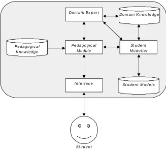
1.1 Architecture of the ITS

(15)

Pedagogical Knowledge

Interface _{Student Models}

Domain Expert

Student Modeller Pedagogical

Module

Student

[image:15.596.148.475.70.365.2]

Domain Knowledge

Fig. 1.1. Traditional architecture of an ITS.

The student modeller develops a representation of the current student using the ITS. This includes long-term knowledge, such as an estimate of the student’s domain mastery, as well as short-time knowledge, such as whether or not the student just violated a rule. Other factors such as motivation can also be modelled, though this is done less frequently. The student modeller will typically save the current student model to the database when the student logs off, and restore it when the student logs back in.

(16)

more time spent revising existing topics the better. The particular method by which this decision is made can be referred to as a pedagogical action selection (PAS) strategy.

Finally, the fourth component of an ITS is the user interface. The user interface is of importance in an ITS. Firstly, it must provide the motivation for the student to continue. If the student lacks the desire to use the system, the ITS simply will not be effective. Secondly, the interface can improve learning significantly by reducing the cognitive load. If only one component of a problem is the focus of teaching, then the rest of the problem can be “externally stored” within the user interface. This means the student does not need to remember extraneous details and can instead target the component of problem-solving that is of importance.

Although all of the components of an ITS are important, it should be clearly obvious that the student model is the most critically important. If the student model is “bad” in that it does not even approximately describe the traits of the current student, then the quality of decisions made by the pedagogical module will be correspondingly bad. This is regardless of the quality of the pedagogical module itself. Considerable research, therefore, has been invested specifically in student modelling.

1.2 The Problem: Uncertainty

(17)

It is relevant to examine the types of uncertainty inherent in student modelling. A student model is constructed from observations that the ITS makes about the student. These can come in the form of responses to questions, answers to problems, traces of the student’s problem-solving behaviour, etc. The student model can in fact be thought of as a compression of these observations: the raw data is combined, some of it may be discarded, and the end result is a summarisation in the form of a set of beliefs about the student. The process of compression is usually defined by a set of inference rules mapping observations to beliefs. However, there are two potential sources of error in this process.

Firstly, the amount of raw data and observations may be insufficient to draw strong conclusions. In the extreme case, one could argue that any data is insufficient unless it can be shown to lead to statistically significant hypotheses. Of course, an ITS rarely has sufficie nt time to acquire enough data to hypothesise about the student’s state to this degree, especially given that the state of the student can be expected to change rapidly.

Secondly, the inference rules for building the student model may themselves be sub-optimal. If the inference rules are inconsistent, incomplete or semantically inexplicable, then the quality of the data will have a reduced bearing on the quality of the resulting student model. In other words, poor inference rules will lead to a poor student model regardless of how reliable or unreliable the data acquired from the student is. But reliable data combined with quality inference mechanisms will lead to a quality student model.

Of course, determining the quality of data and inference rules is not a simple task. One can never guarantee that the data is truly representative of the current state of the student; it may just be random noise. Thus, building the student model is a highly uncertain activity.

(18)

of actions being selected that are not optimally adapted to the student. However, if the student model is of a relatively high quality and the action selection functions are insensitive to small amounts of uncertainty, it may well be the case that the selected actions remain optimally near-optimally rational. Unfortunately, it is difficult to determine the degree of rationality of the action selection function, especially when the rules defining the function are not based on theory. In a hypothetical worst case, the action selection functions could make random decisions. Typically, however, the action selection function will be some heuristic that considers the values in the student model (e.g. one such heuristic is to give a hint on the rule that the student has most frequently violated in the past), though such an approach cannot guarantee that this is the best possible rule. This type of uncertainty, as well as the uncertainty inherent in the student model, can contribute to overall sub-optimal behaviour in the ITS.

Observation

Teaching

Actions Student Model

Weak Inference Rules and Noisy Data

à Uncertainty (1st Type)

Sub-optimal Action Selection Rules

à Uncertainty (2nd Type) Student

responses

Fig. 1.2. Sources of uncertainty in an ITS.

(19)

1.3 Towards A Solution: Normative Theories

The question that arises is how to minimise uncertainty. It is very difficult, if not impossible, to eliminate uncertainty of the first type. While the inference rules for building the student model may be optimised (and there is much research in this area), there is no way to guarantee the quality of the data. Uncertainty of the second type (which occurs because of sub-optimal action selection), however, presents a different challenge. Powerful general theories of decision- making, designed specifically for situations involving uncertainty, have been developed. One of them is Bayesian probability theory (Bayes, 1763), which deals with uncertain reasoning, and the other is statistical decision theory (Savage, 1954) that extends Bayesian probability to making decisions and incorporates a measure of preference for the outcomes of actions called utility. If the tenets of these theories are accepted (and to date there have been no substantial reasons why they should not be), then the theories define rationality. It is a challenge to ITS researchers, then, to define action selection functions based solely on these theories for incorporation in their systems. Doing so would eliminate uncertainty of the second type and make their systems more acceptable (i.e. more rational) in the process. A consequence of this is that when an ITS does exhibit irrational behaviour, the cause can be traced uncertainty of the first type rather than of the second.

To describe in more detail exactly how to produce a normative ITS, a general methodology is introduced in this thesis. The methodology uses machine learning and statistical significance tests to construct a Bayesian network student model from student performance data. It describes how to integrate this model with decision-theoretic procedures for PAS. A critical component of the methodology is evaluation in a real classroom. All too frequently, ITSs are evaluated only in the lab and never make it to the classroom. However, classroom evaluation is essential in order to obtain valuable data which can guide the further development of the system.

(20)

reasoning under uncertainty. When normative theories are referred to as “optimal” in this thesis, it is meant that given a scenario defined as a probability distribution and a utility function, then a normative system can reason and behave optimally within the confines of the scenario. Normative theories themselves are independent of the scenario semantics. For example, although Bayesian probability theory provides all the mechanisms for representing and reasoning about uncertain knowledge, it does not specify what the knowledge that is being reasoned about actually is. That is the domain of psychological learning theories. To further clarify this, consider that a particular learning theory may be implemented in two different ways: with normative methods, or using an ad-hoc representation such as heuristic rules. If the learning theory is precisely defined, the normative implementation will guarantee that the learning theory is optimally applied to the student in the sense that it is rational, but the ad-hoc implementation may be sub-optimal.

1.4 Demonstrations of Normative ITSs

The effectiveness of normative theories was evaluated in the classroom using two different ITSs. The first system, SQL-Tutor (Mitrovic & Ohlsson, 1999), is an existing ITS for teaching the SQL database language to computer science undergraduate students. Domain knowledge is represented in the form of constraints (Ohlsson, 1994) that specify the form of consistent or correct solutions. For its long-term student model, SQL- Tutor originally had a simple frequency-based overlay model. A Bayesian overlay model replaced this (Mayo & Mitrovic, 2000), and a new method of next problem selection was the implemented. This latter version of SQL-Tutor was evaluated in October 1999.

(21)

sophisticated than the simple Bayesian overlay in SQL-Tutor. CAPIT’s student model was constructed by application of the methodology described in this thesis. As a consequence, it has a sophisticated, adaptive Bayesian network that can model complex interdependencies between student performance and the domain constraints. The output of the Bayesian network (which is a prediction about how the student will be behave in a given context) is the input to a decision-theoretic process for tutorial action selection. Effectively, CAPIT’s entire mechanism for representing and reasoning about the student, and determining its own behaviour, is normative.

CAPIT was fully evaluated in the classroom over a period of four weeks during June 2000. Three classes participated in the evaluation. One of the classes did not have access to CAPIT and use used as a baseline for comparing the pre- and post-test results; the second used a “randomised” non- normative version of CAPIT, and the third class used the normative version of CAPIT. Both classes using CAPIT improved from pre-test to post-test. The pre- and post-tests, and the log file analysis, indicate that the class using the normative version of the system learned the constraints at a faster rate than the class using the randomised version.

1.5 Guide to the Thesis

(22)

(23)

11

Chapter 2

Bayesian Networks and Decision Theory

Both Bayesian probability theory (Bayes, 1763) and statistical decision theory (Savage, 1954) are instances of normative systems. A normative system is a set of rules as well as the logical consequences of those rules (Gardenförs, 1989). Therefore, if logical reasoning and behaviour are assumed to define rationality, a normative system can be considered a model of rational behaviour. This implies that, given a specific normative model, the output from a normative system will be optimal for that model. Heuristic or ad-hoc systems cannot guarantee this because the inferences do not have to be logical consequences, and therefore they can be incomplete or inconsistent.

(24)

of actions. It provides a method of “fusing” preferences with beliefs to give a measure on possible actions called the expected utility.

One aspect of normative systems is that because they are prescriptive, they specify what to compute for logical/rational behaviour (the prescriptive requirement) rather than how to compute it (the implementation). As a result, considerable research in recent times has been directed at the development of sophisticated algorithms for implementing normative reasoning (e.g. Lauritzen & Spiegelhalter, 1988). All the algorithms compute the same thing – they adhere to the tenets of the normative system – but their efficiencies vary considerably and depend to greater and lesser extents on the particular domain being modelled.

This chapter aims to give the reader a firm grounding in Bayesian and decision-theoretic technology. Detailed descriptions are given of the algorithms used both in the construction of CAPIT (specifically, the Bayesian network induction algorithms) and during the execution of CAPIT (the Bayesian network reasoning algorithm and the decision-theoretic expected utility formula). Although complete understanding of the algorithms and mathematics is not necessary to appreciate the main results of the thesis, the details are included because they provide the foundation of the CAPIT tutoring system described later. Taking the time to absorb these algorithms will give the reader an appreciation of how normative approaches to knowledge representation and reasoning differ from other approaches. The most significant mathematical results will be reiterated at the end of this chapter.

(25)

2.1 Probability Basics

Bayesian probability theory deals with events and the probabilities of those events. If A is an event, then the probability of A is denoted by a real- valued number, P(A). The basic axioms of probability theory (Bayes, 1763; Cowell, 1999) are:

1. P(A) = 1 if and only if A is certainly true.

2. P(A) = 0 if an only if A is certainly false.

3. 0 = P(A) = 1.

4. If A and B are mutually exclusive, then P(A ∪B) = P(A) + P(B).

It is pertinent to define a particular class of events, that of a variable X being with certainty in one and only one of the discrete states x1..xn. We denote

the probability of this event by P(X=xi), and it follows from the axioms that:

1 1

)

( =

∑

= =

n

i i

x X

P (2.1)

The sequence of probabilities P(X=x1), P(X=x2), …, P(X=xn) define a

probability vector. A useful shorthand way of referring to this vector is simply P(X).

An important concept is that of the conditional probability, P(X=x|Y=y) = r. This represents the statement “If Y=y is true, and no other information to hand is relevant to X, then the probability of X=x is r.” A table defining conditional probabilities for every possible combination of values that X and Y can take is called a conditional probability distribution and is denoted by P(X|Y).

Conditional probabilities are essential to a fundamental rule of probability calculus, the product rule. The product rule defines the probability of a conjunction of events:

(26)

Frequently, the literature shortens P(A ∩ B) to P(A,B), and that convention will be followed here. P(A,B) is also called a joint probability distribution, and like the conditional probability distribution, it is a table of values, one entry for each possible combination of values that its variables can jointly take. In the general case, a joint probability distribution over n variables can be defined recursively using the product rule (Equation 2.3):

P(X1, X2,…, Xn) = P(X1| X2,…, Xn)P(X2,…, Xn)

= P(X1| X2,…, Xn)P(X2| X3,…, Xn)P(X3,…, Xn)

= P(X1| X2,…, Xn)P(X2| X3,…, Xn)….P(Xn-1|Xn)P(Xn) (2.3)

This property of joint probability distributions is called the general factorisation property. Note that the product rule allows any ordering of variables in the factorisation.

Rearranging the product rule leads to Bayes’ famous theorem:

) ( ) ( ) | ( ) | ( B P A P A B P B A

P = (2.4)

Bayes’ Theorem is frequently used for reasoning about an uncertain hypothesis A given evidence B, and in that context P(A|B) is called the posterior probability of A, P(A) is called the prior probability of A, and P(B|A) is the likelihood of A. The factor

) ( 1

B

P is a normalisation constant, and if ignored,

Bayes’ Theorem simplifies to:

P(A|B) ∝ P(B|A)P(A) (2.5)

This form of Bayes’ Theorem is important because frequently the normalisation step can be left until the very end of a chain of calculations, making the computations more efficient.

(27)

X2, …, Xz} and a joint probability distribution P(X) (equivalent to P(X1, X2, …,

Xz)), then we can find the sub-joint probability distribution P(Xq) for any Xq ⊆

X by applying the marginalisation rule:

∑ =

−Xq X

X q

X ) ( )

( P

P (2.6)

This rule is effectively a summation over the variables that are not of interest (those being X-Xq), so the joint probability distribution collapses to a

distribution over only those variables of interest (Xq). For example, suppose we

have the joint probability distribution P(A,B,C) and we want to marginalise A. If B and C are binary (taking values Y or N), then using Equation 2.6 to calculate P(A) leads to the following calculation:

P(A) = P(A,B=Y, C=Y) + P(A,B=Y, C=N)

+ P(A,B=N, C=Y)+ P(A,B=N, C=N) (2.7)

This completes the definition of the basic concepts of probability theory. Conditional and joint probability distributions have been defined, and it has been shown how joint probability distributions can be both constructed using the product rule and reduced via marginalisation. Bayes’ Theorem, a rule crucial for Bayesian reasoning under uncertainty, has been introduced.

2.2 Bayesian Network Basics

A significant efficiency issue that any implementation of Bayesian probability theory must deal with is storage requirements. To illustrate, an explicit table representation of P(X1, X2,… ,Xn) will, if n=16 and each Xi is binary, require 216

(28)

probability distribution or a subjoint distribution thereof. This way, the entire joint probability distribution table would not need to be explicitly represented. For example, if we wished to determine an entry from a subjoint distribution, say P(X2=x2,X3=x3), we could simply evaluate the function f(X2=x2,X3=x3),

instead of marginalising P(X2,X3) from P(X1, X2,… ,Xn) and then looking up the

appropriate entry in P(X2,X3).

The representation of P(X1, X2,… ,Xn) as a factorisation of n-1

conditional probabilities and one probability vector (Equation 2.3) is a possible definition of f. Instead of representing the entire joint probability table explicitly, we represent each factor separately and multiply appropriate entries from each factor’s table every time f is evaluated. This would be very efficient for some queries, such as P(Xn=xn), which is represented explicitly, and P(Xn-1=

xn-1, Xn=xn), which can be computed with a single multiplication using the

product rule, but for other queries like P(X1=x1), the new representation will be

no more efficient. Ideally, the factors should be compressed even further.

One approach to achieving this is to look for a certain property of the conditional probability tables P(X1|X2…Xn), etc, called conditional

independence. To illustrate conditional independence, consider the smaller joint distribution P(A,B,C). The product rule and the general factorisation property mean that we can express this as:

P(A,B,C) = P(A|B,C)P(B|C)P(C) (2.8)

Now, suppose that the factor P(A|B,C) has the property that it is always equal to P(A|C). That is, for every pair (a,c), P(A=a|B,C=c) remains constant as B varies. We therefore say that A is conditionally independent of B given C. In standard notation, this is expressed as:

C B

AC | (2.9)

We can therefore drop B from the conditional probability P(A|B,C) altogether and rewrite the representation as:

(29)

Storage-wise, this new representation is more efficient than Equation 2.8. That is, if A, B and C are binary, then the factor P(A|B,C) which requires 23 entries has been replaced by the factor P(A|C) requiring only 22 entries.

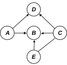
Because of the efficiency gains that conditional independence gives us, Bayesian networks were developed to make the conditional independencies explicit. In a Bayesian network, a variable that conditions another variable in the factorisation (e.g. C conditions A and B in Equations 2.8 and 2.10, and B conditions A in Equation 2.8), becomes the parent of that variable in the network. It makes no sense to have directed loops in the network because this would represent a factorisation impossible to derive from the product rule. A Bayesian network, therefore, is a directed acyclic graph. Figure 2.1 depicts a Bayesian network for the distribution defined in Equation 2.8, and Figure 2.2 depicts a network for the more efficient representation defined by Equation 2.9.

A B

C

Fig. 2.1. A Bayesian network for P(A,B,C) = P(A|B,C) P(B|C)P(C)

A B

C

Fig. 2.2. A Bayesian network for P(A,B,C) = P(A|C) P(B|C)P(C)

The key advantage Bayesian networks give us is the ability to define the conditional independencies first, before specifying numerically the actual conditional probability distributions.

(30)

) PA( )

ND(X X

XC | (2.11)

That is, if a variable’s parents become known, then any more information about nodes that are not on a directed path from X will be irrelevant. This is the so-called directed Markov property of Bayesian networks. It effectively sets bounds on the influence of new evidence, an important consideration for efficient inference that will be discussed in more detail later.

The question arises as to how to use the directed Markov property to reduce the size of a general representation such as the factorisation in Equation 2.3. Now, the product rule does not limit the order in which variables are factorised, so therefore if an ordering of nodes can be found such that each variable in the factorisation is conditioned on only its parents and its non-descendents, then the non-descendents will “drop out” of the equation and each variable will be conditioned only on its parents. That is, we want to use conditional independence to simplify Equation 2.3 to:

P(X1, X2,…, Xn) = P(X1| PA(X1))P(X2| PA(X2))….P(Xn| PA(Xn))

=

∏

=

n

i

i X

X P

1

) |

( PA( ) (2.12)

It happens that a suitable ordering of nodes X1, X2,…, Xn will always

exist in a Bayesian network, and that ordering is called a topological ordering. A relatively simple algorithm can find the topological ordering (Cowell, 1999): initialise an empty list, then iteratively delete from the network any variable with no parents, and append it to the end of the list until all the variables have been appended. The list will then be a topological ordering of the nodes from which Equation 2.12 can be defined. Equation 2.12 is also known as a recursive factorisation, and is a standard method of numerically representing a Bayesian network. Note that a recursive factorisation corresponds to the topology of the Bayesian network, as there is one factor for each node and its parent set.

(31)

represent P(X1,…,X16). Now however, if each variable is on average dependent

on only two parents, then an average of 23 = 8 conditional probabilities per factor need to be stored. This means that the entire joint probability distribution (specified by Equation 2.12) can be specified by approximately 8n = 128 entries, a considerable saving. Of course, the size of the specification will increase as the number of dependencies increases, but, in practice, real-world Bayesian networks are sparsely connected and therefore they benefit from this representation.

While conditional independence is highly advantageous for specifying a Bayesian network compactly, Equation 2.12 does not capture all the conditions under which variables within a network are independent. More generally, two variables are d-separated if evidence about one cannot influence the other. To determine whether or not two nodes are d-separated, one must consider all the undirected paths between the two nodes. Any node on any of the paths may “block” the dependence along that path, and therefore if all the paths between the two variables are blocked at least once, the two nodes will be independent (i.e., d-separated). The smallest set of nodes that d-separates two nodes X and Y is called the cut-set of X and Y (Pearl, 1988).

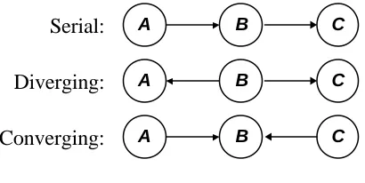
Consider a node on a path in the Bayesian network. There are three classes of connection along that path: serial, diverging, and converging, and they are depicted in Figure 2.3.

Serial: A B C

Diverging: A B C

[image:31.596.227.432.525.628.2]

Converging: A B C

Fig. 2.3. Serial, diverging and converging connections to a node B on a path.

(32)

special case of A being conditionally independent of its non-descendents given its parents, and is equivalent to Figure 2.2.

The interesting case is that of the converging connection. If A and C converge to B, it transpires that they will be d-separated as long as B and none of B’s descendents are observed; if B or one of its descendents are observed, A and C become dependent. This interesting property of converging connections arises because A and C represent multiple explanations or causes of the converging node B. For example, suppose A is the proposition that Student X has mastered the topic and C is the proposition that Student X performs poorly on exams. If B is the proposition that Student X failed the exam, then A and C are two possible explanations for B and would therefore converge to B in a Bayesian network. If we subsequently observe B (say, to find that the proposition is true and the student did fail the exam), then B’s causes become dependent because if A is subsequently observed to be true as well, then it (intuitively) has some bearing on C (we might revise the probability of C downwards) and vice versa.

Thus, d-separation characterises independence arising from lack of evidence as well as evidence. Note that any system for reasoning under uncertainty must capture these properties, as they are basic attributes of human reasoning (Jensen & Lauritzen, 2000).

(33)

2.3 Inference in Multiply-Connected Bayesian Networks

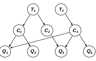
Inference is the general problem of computing the posterior probability P(Q|E=e), for some evidence E=e and query Q (where Q ⊆ X and E ⊆ X). We defined the posterior probability using Bayes’ Theorem (Equation 2.4) in the previous section, but the problem is how to calculate this quantity efficiently. To illustrate how the naïve approach is inefficient, consider the Bayesian network depicted in Figure 2.4 and its recursive factorisation, Equation 2.13. The Bayesian network is a simple and contrived student model in which a student’s mastery of the domain topics (T1 and T2) implies her mastery

of the various concepts (C1..C3), which in turn influences her performance on

test questions (Q1..Q4). The questions may require the student to have mastered

more than one concept. With this Bayesian network, we can perform inferential queries, such as P(Q1|T1=Mastered); diagnostic queries such as

P(T2|Q3=Failed); or a combination of both, such as P(C2|Q4=Correct,

T1=Not-Mastered).

Q1 Q2 Q3

T1

C2 C3

Q4

C1

[image:33.596.217.411.440.564.2]

T2

Fig. 2.4. Graphical structure of a Bayesian network.

P(X) = P(Q1|C1,C3)P(Q2|C1)….P(C1|T1)…P(T1)P(T2) (2.13)

(34)

even the simplest query, the marginalisation steps require summations and multiplications over all the variables in the network.

A more efficient approach utilises conditional independence and the topology of the Bayesian network to perform a series of more efficient local, rather than global, computations. Local computation in a Bayesian network is the process of computing a variable’s posterior probability distribution from the posterior distributions of its neighbours – and only its neighbours. Thus, when evidence arrives at a node, its neighbours update themselves, then their neighbours update themselves, and so on, until the entire network “absorbs” the evidence. This process is analogous to propagation in a neural network, except that it is probabilistic consistency, as opposed to “activation”, that spreads across the network.

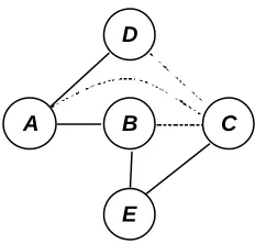
Inference via local computation is highly efficient for singly-connected Bayesian networks (Pearl, 1988). Various algorithms with propagation time proportional to the number of variables in the network are described by Pearl (1988) and, specifically for implementation in an ITS, Murray (1999). However, the situation is more complex when the network is multiply-connected, because there are loops in the underlying undirected graph. To illustrate, consider Figure 2.5.

B C

A

D

Fig. 2.5. A Bayesian network for P(A,B,C,D) = P(D|B,C)P(B|A)P(C|A)P(A)

(35)

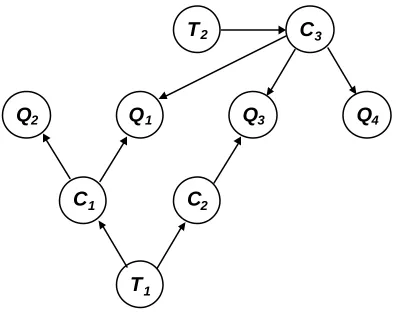
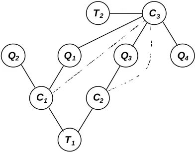
singly-connected networks because there is always at most one path between any two variables, but singly- connected networks are highly restrictive and not suitable for many domains. For example, even the simple Bayesian network depicted in Figure 2.4 is multiply-connected, as can be seen from an isomorphic rearrangement of the nodes depicted in Figure 2.6.

Q1 Q3

Q2

T₁ C₂

C3

Q4

C₁

[image:35.596.214.413.194.350.2]

T2

Fig. 2.6. The same Bayesian network as depicted in Figure 2.4, but with its nodes

rearranged to make the undirected cycle T1-C2-Q3-C3-Q1-C1 explicit.

We therefore present a general algorithm for inference in multiply-connected Bayesian networks. The algorithm was introduced by Lauritzen & Spiegelhalter (1988) and further clarified by Jensen, Lauritzen et al. (1990) and Jensen, Oleson et al. (1990). It is most recently described in Jensen & Lauritzen (2000). Cowell et al. (1999) provides a tutorial introduction and overview of the algorithm for Bayesian network novices. The algorithm is a cornerstone for exact Bayesian network inference. Numerous variations (e.g. Kjaerulff, 1999) have since been proposed since in the literature, and the algorithm has been implemented in most of the common Bayesian network shells, e.g. HUGIN (Andersen, Oleson, et al., 1989), SMILE/GENIE (on World Wide Web at http://www2.sis.pitt.edu/~genie/), and MSBN (http://research.microsoft.com/ msbn).

(36)

having two stages: a compilation stage, in which the input is the original Bayesian network specification and the output is the singly-conne cted structure, and a propagation stage, in which evidence is absorbed and queries are performed on the new structure. If the network specification changes, compilation must occur again to produce an updated singly-connected structure before further querie s can be performed.

Another way of considering the algorithm is to think of two parallel processes; one graphical, in which the network structure is manipulated, and one numerical, in which the probabilities are manipulated. The numerical calculations always correspond to the graphical operations. Figure 2.7 depicts the architecture and functionality of the algorithm from these viewpoints. The details of this diagram will be explained in the following sub-sections.

P(Q|E) Compilation

Propagation

Evidence E

Query Q

Definition P(X)

∏₌

=n 1 i

i i|pa(X))

P(X ) P(X

A

B C

D

A B C B,C B C D ∏

= =m 1 i i) BEL(C ) BEL(X

A B C B,C B C D

∏ = = m 1 i i 0 0₍ ₎ _BEL_(C₎

BEL X ∏ = = m 1 i i 1 1₍ ₎ _BEL_(C₎

BELX

Evidence arrives at, e.g., D…

…and propagates to A via B and C

Fig. 2.7. Overview of the L & S algorithm.

2.3.1 Graphical Compilation

(37)

Step

1 Marry co-parents. 2 Moralise network. 3 Triangulate network.

[image:37.596.214.411.425.578.2]

4 Form junction graph of cliques. 5 Form junction tree.

Table 2.1. Steps required to generate a junction tree.

The first two steps are relatively straightforward. The marrying of co-parents is the simple addition to the directed network of an edge between any two nodes that are parents of the same child, but not already neighbours. The moralisation of the network is the dropping of all directionality. That is, the directed network is turned into an undirected graph. The output of these two steps when applied to the example Bayesian network in Figures 2.4 and 2.6 is shown in Figure 2.8. The only non-adjacent co-parents in the original network are (C1, C3), and (C2, C3), and so edges between these pairs are added to the

network. (The new edges are dashed in Figure 2.8.)

Q1 Q3

Q2

T1

C2

C₃

Q4

C1

T2

Fig. 2.8. The married, moralised graph.

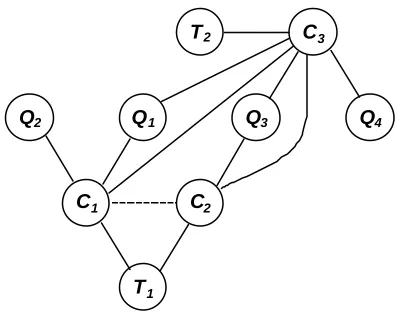
The next step is triangulation: “short cuts” (or, in graph-theoretic terminology, chords) are successively added to every cycle of length 4 or more that does not already have a chord, until no such cycles exist. To illustrate, consider Figure 2.8. A number of cycles exist in this graph, such as Q1-C3-C1

and C3-C1-T1-C2-Q3. However, neither of these are candidates for shortening

(38)

has a chord, C2-C3. In fact, there is only one cycle in Figure 2.8 appropriate for

shortening, and that is the cycle C3-C1-T1-C2. There are two possible chords that

could shorten this cycle: C1-C2 or T1-C3. In both cases, the new edge renders the

graph fully triangulated. We have chosen to add the edge C1-C2, and the result is

depicted in Figure 2.9. (An exact algorithm for triangulating the network will be discussed later.)

Q1 Q3

Q2

T1

C2

C3

Q4

C1

[image:38.596.184.383.213.370.2]

T2

Fig. 2.9. The triangulated graph.

The fourth step involves firstly identifying the cliques in the triangulated graph, and secondly forming a new graph called a junction graph. A clique is a graph-theoretic concept defined as a “maximal, complete” subgraph. A subgraph is complete if every node in the subgraph is adjacent to every other node. For example, {C1,C2,T1} is a complete subgraph in Figure 2.9, but

{C3,Q3,Q4} is not because there is no edge Q3-Q4. The maximal property adds

the criterion that one cannot find another node in the network to add to the subgraph such that the subgraph will still be complete. In other words, {C1,C2,T1} is maximally complete because there is no other node that can be

included in this subgraph whilst maintaining the completeness property. However, {C1,C3} is complete but not maximally so because {C1,C3, Q1}, the

subgraph formed by adding Q1, is complete. The cliques of Figure 2.9,

therefore, are: {T2, C3}, {C3, Q4}, {C1, C2, C3}, {C2, C3, Q3}, {C1, Q2}, {C3, Q1,

C1}, and {C1, C2, T1}.

(39)

Furthermore, variables from the original graph are likely to appear in more than one clique; to capture this in the junction graph, an edge is added between two cliques if their intersection is non-empty. Figure 2.10 is the junction graph derived from Figure 2.9.

C1 C2 T1 C2 C3 Q1

C₁ Q₂ C₂ C₃ Q₃

T2 C3

[image:39.596.185.438.624.735.2]

C₁ C₂ C₃ C3 Q4

Fig. 2.10. The junction graph.

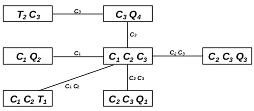
Recall that the motivation for the compilation stage is to produce a singly-connected structure on which inference via local computation is possible. This structure, the junction tree, is formed by simply “pruning” the junction graph until only a tree remains (see Section 2.3.5 for an algorithm that does this). However, the junction tree has an additional property not present in the junction graph; namely, the running intersection property: if any two cliques in the junction tree contain a mutual variable X from the original network, then every clique on the path between those two cliques must also contain X. This ensures that the junction tree does not have two or more disconnected “representations” of the same variable. The running intersection property thus restricts the way in which a junction graph can be “pruned” to a junction tree. A junction tree for Figure 2.10, with the clique intersections labelling the edges, is depicted in Figure 2.11.

C1 C2 T1 C2 C3 Q1

C1 Q2 C2 C3 Q3

T2 C3

C1 C2 C3

C3 Q4

C2 C3

C2 C3 C1 C2

C1

C3 C3

(40)

2.3.2 Numerical Compilation

A logical mapping exists between the original form of a Bayesian network and its recursive factorisation. For each variable X, there is one and only one factor P(X| PA(X)) in the recursive factorisation. Now that the original network has been converted into a junction tree, a new numeric representation with a logical mapping between cliques and factors can be derived. More specifically, if C is the set of cliques in the junction tree, a suitable new representation is:

P(X1, X2,…, Xn)=

∏

=

n

i

i X

X P

1

) |

( PA( ) =

∏

∈C C

i C

i

P( ) (2.14)

where P(Ci) is called a clique marginal, which is simply a joint probability

distribution over the variables in the clique.

One important change in the processing from now on is that beliefs rather than probabilities will be computed. A belief is equivalent to a probability, with the exception that individual beliefs are allowed to exceed 1, and there is no ensuing requirement that the entries in a belief table or vector must sum to unity. When beliefs are utilised, the relative rather than absolute differences between values becomes important. Other than that, beliefs and probabilities are identical. Beliefs allow for slightly more efficiency in the processing because the tables do not need to be normalised after each calculation. A belief table, denoted by BEL, can always be transformed into a probability table by dividing every entry in the belief table by the normalisation constant Z, i.e.:

P(X) = Z-1BEL(X) (2.15)

(41)

P(X1, X2,…, Xn) ∝ BEL(X1, X2,…, Xn) =

∏

∈C C

i C

i

BEL( ) (2.16)

The process by which the clique marginals BEL(C1) etc., are derived

from the original conditional probabilities is straightforward and involves rearranging the terms of the recursive factorisation. Cowell et al. (1999, pp. 34) define an algorithm to achieve this, which is given in Listing 2.1. The algorithm transforms the recursive factorisation into a potential representation, from which the clique marginals can easily be derived via marginalisation.

• For each clique Ci ∈ C, define a function ai(Ci).

• Initialise ai(Ci) := 1 for each Ci.

• For each factor P(X|PA(X)) in the recursive factorisation:

o Find one clique Ci containing both X

and PA(X) and redefine ai(Ci) :=

ai(Ci)P(X|PA(X)).

List. 2.1. Defining a potential representation from a recursive factorisation (Cowell et

al., 1999, pp. 34)

More mathematical details of this process are available in Lauritzen & Spiegelhalter (1988) and Jensen et al. (1990).

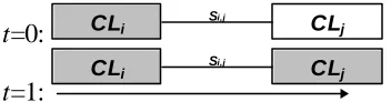
2.3.3 Graphical Propagation

(42)

consisting of two cliques. The evidence arrives at CLi and propagates to CLj in

one time step.

t=0: CLi Si,j CLj

t=1:

CLi CLj

[image:42.596.197.373.133.179.2]

Si,j

Fig. 2.12. Evidence arrives at CLi at time t=0, and CLj calibrates itself to CLi at time

t=1.

Propagating single pieces of evidence is relatively simple and this process could be used to sequentially propagate multiple pieces of evidence. However, a major advantage of the L & S algorithm is that multiple evidence items can be propagated on a junction tree simultaneously, and therefore much more efficiently (especially for parallel-processor implementations of the algorithm, e.g. Kozlov & Pal Singh (1994)). Figure 2.13 depicts a case where evidence is propagating to a single clique CLj from two of its neighbouring

cliques, CLi and CLk.

t=0: CLi Si,j CLj Sj,k CLk

t=1:

CLi CLj

Si,j

CLk Sj,k

t=2:

CLi CLj

Si,j

CLk Sj,k

Fig. 2.13. Evidence arrives at CLi and CLk at time t=0. CLj calibrates itself to both CLi

and CLk at time t=1, then CLi and CLk calibrate themselves to CLj at t=2.

(43)

CollectEvidence in all of its neighbours, then calibrates itself to them. Using these simple methods, this approach to Bayesian reasoning can be easily conceptualised.

2.3.4 Numerical Propagation

The numerical formulation of propagation consists of two rules for updating clique marginals: a simple rule for propagating evidence from one clique to another, and a more ge neralised rule for absorbing multiple evidence. Both rules are derived from the product rule.

Let BELt(X) denote the belief distribution over variables in set X at time t. Consider two adjacent cliques in the junction tree, CLi and CLj. Now, CLi

and CLj must have a non-empty intersection in order to be adjacent, and that

intersection can be defined as another set:

Si,j = CLi∩ CLj (2.17)

Si,j is called the separator of CLi and CLj. Now consider the remainder of both

cliques when the separator is subtracted:

Ri = CLi – Si,j, Rj = CLj – Si,j (2.18)

Ri and Rj are called the residuals.

Because a clique can be viewed as the union of the residuals and separators, a clique marginal can be defined by the product rule as:

BELt(CLi) = BEL t

(Ri, Si,j) = BEL t

(Ri|Si,j)BEL t

(Si,j) (2.19)

and by marginalisation, we can compute the subjoint belief over the separators from the joint belief over the clique:

BELt(Si,j) =

∑

− i,j i S CL

i CL ) (

t

(44)

Note that we can apply Equation 2.20 to both of the cliques CLi and CLj

to get BELt(Si,j). Therefore, to indicate from which clique the distribution over

separators was computed, a subscript i is used. For example, BELt_i(S_i,_j) indicates a distribution computed by applying Equation 2.20 to the belief over the ith clique, BELt(CLi), and not the jth clique, BELt(CLj).

Given that two neighbouring cliques CLi and CLj can both compute

belief distributions over their common separators, we say they are consistent if )

(Si,j t i

BEL =BELt_j(S_i,_j), and inconsistent if BELt_i(S_i,_j)? (Si,j) t

j

BEL . Ideally, they should always be consistant. However, if evidence arrives at one clique but not its neighbouring cliques, then that clique will become inconsistent with its neighbours. To absorb the evidence, the neighbouring cliques make themselves consistent via calibration. Thus, “propagation” or “evidence absorption” in a junction tree is the successive calibration of cliques to ensure consistency.

Calibration of a single item of evidence is a relatively simple process. Suppose evidence arrives at clique CLi at t=0, as in Figure 2.12. BEL0(CLi) is

the posterior belief distribution over the clique given the evidence, but so far its neighbour has not been updated. Therefore, CLj will be inconsistent with CLi

and must calibrate.

By Equation 2.19, BEL0j(Si,j) is a factor of BEL 0

(CLj). To calibrate, we

essentially replace BEL0_j(S_i,_j) in the factorisation with BEL0_i(S_i,_j), and compute the new belief distribution over the clique, BEL1(CLj). That is, we delete the

factor reflecting that state-of-affairs prior to the evidence (BEL0_j(S_i,_j)), and insert an equivalent factor that does incorporate the evidence (BEL0_i(S_i,_j)). This new factor also makes the cliques consistent. The entire operation can be captured by a single equation:

) ( ) ( ) ( )

( ₀ 0

0 1 j i, j i, j j S S CL CL i j BEL BEL BEL

BEL = (2.21)

(45)

A generalisation of Equation 2.21 is used to update a clique (e.g. CLj)

when evidence arrives at more than one of its neighbours (e.g. CLi and CLk), as

in Figure 2.13. To do this, the separators between the clique and each of its neighbours must be considered. (In this example, the separators are Si,j and Sj,k.)

The update rule allowing CLj to absorb evidence from both sources

simultaneously is a generalisation of Equation 2.21:

) ( ) ( ) ( ) ( ) ( )

( 0 0

0 0 0 1 k j, j i, k j, j i, j

j S S

S S

CL

CL _i _k

j j BEL BEL BEL BEL BEL

BEL = (2.22)

Now that CLj has been updated, it will still be inconsistent with its

neighbours because the evidence from CLi has not propagated to CLk and vice

versa; it has only got as far as CLj. The final step is to apply Equation 2.21 to

calibrate CLi and CLk to CLj:

) ( ) ( ) ( )

( ₀ 1

0 2 j i, j i, i i S S CL CL j i BEL BEL BEL

BEL = , ( )

) (

) ( )

( ₀ 1

0 2 k j, k j, k k S S CL CL j k BEL BEL BEL BEL = (2.23)

To summarise, the numeric propagation part of the L & S algorithm is basically the propagation of consistency from a clique to its neighbours in a junction tree (a process called calibration). Consistency is a property belonging to pairs of neighbouring cliques, and is achieved when marginalising on the variables shared by both neighbours yields the same belief distribution.

Finally, the last step by which a general query P(Q|E=e) is calculated will be mentioned. We have already shown how the junction tree absorbs the evidence E=e. The final step is to find one or more cliques containing the variable(s) Q, and marginalise BEL(Q) from them. BEL(Q) can then be normalised to yield the posterior probability distribution over Q.

2.3.5 Efficiency and Implementation Issues

(46)

construction (Step 5). In this section, some algorithms for graph triangulation and junction tree construction are described.

Graph triangulation has long been known to be an NP-Hard problem (Yannakakis, 1981). As a result, considerable research has been undertaken to develop heuristic, near-optimal solutions. One common approach is called one-step look ahead triangulation (Cowell et al., 1999) and is shown in Listing 2.2. Basically, this approach takes each node and its neighbours, and “fills in” edges between them to form a completely connected subgraph in the network.

Note that the order in which nodes are numbered depends on a user-defined crit erion, c(V). Nodes can be selected to maximise or minimise this quantity. While the algorithm is relatively straightforward, its efficiency and the quality of the resulting triangulation will depend on how c(V) is defined. Cowell et al. (1999, pp. 58) suggest that c(V) be set to the size of the subjoint distribution over V and its neighbours, and therefore the function should be minimised.

• Start with all vertices unnumbered.

• Set i := n, where n is the number of nodes in the graph.

• Do until there are no more unnumbered vertices:

o Select an unnumbered node V that

optimises the criterion c(V).

o Number it with i (i.e. set Vi := V).

o Form the set Ci consisting of Vi and

its neighbours in the graph.

o Add edges between the nodes in Ci to

make Ci a complete subgraph.

o Decrement i.

List. 2.2. One-Step Look Ahead Triangulation (Cowell et al., 1999, pp. 58).

(47)

ahead is unnecessary. Maximum cardinality search, given in Listing 2.3, is an algorithm for determining whether or not a graph is triangulated. It is a highly efficient algorithm that operates in O(n+e) time, where n is the number of nodes and e is the number of edges in the network. Note that ne(V) is a function returning V’s neighbours in the network, but excludes V itself.

• Set Output := “Graph is Triangulated”. • Set i := 1.

• Set L := {}

• Set V to all the nodes in the network. • For each node V ∈ V, set c(V) := 0.

o Do while L ? V:

o Set U:=V-L

o Select any V from U maximising c(V) and

number it i (i.e. set Vi := V)

o Set Pi := ne(Vi) n L.

o If Pi is not a complete subgraph, Then:

Set Output = “Graph is not

triangulated”.

Else

Set c(W)=c(W)+1 for each W ∈

ne(Vi) n U.

o Set L := L ∪ {Vi}

o Increment i.

• Report Output.

List. 2.3. Maximum Cardinality Search (Cowell et al., 1999, pp. 55).

Besides determining the triangulatedness of a graph, maximum cardinality search also provides a useful numbering of the nodes V1…Vk. This

(48)

CL1... CLp for the junction graph, but also a particular numbering of those

cliques that is useful for building the junction tree from the junction graph..

• Start with the node numbering V1…Vk and the sets P1…Pk obtained by maximum cardinality

search.

• Denote the cardinality of Pi by pi.

• Call Vi a “ladder node” if i=k or if i<k and

pi+1<1 + pi.

• Denote the jth ladder node, in ascending

order, by λj.

• Define the clique CLj = {λj} ∪ P(λj).

List. 2.4. Finding the Cliques of a Triangulated Graph (Cowell et al., 1999, pp. 56).

The ordering of the cliques produced by Listing 2.4 is crucial for the final algorithm presented here: junction tree construction. Listing 2.5 shows how to construct such a junction tree from the cliques and the clique ordering. Other algorithms for finding the optimal junction tree have been proposed by Jensen & Jensen (1994) and Kjaerulff (1992).

• Associate a node of the tree with each clique CLi.

• For i=2..p, add an edge between CLi and CLj

where j is any one value in {1,…,i-1} such

that CLi ∩ (CL1 ∪ CLi-1) ⊆ CLj.

List. 2.5. Junction Tree Construction (Cowell et al., 1999, pp. 55).

(49)

becomes easier to find the cliques and construct a junction tree with the running intersection property, as demonstrated by the relatively simple algorithms shown in Listings 2.4 and 2.5.

2.3.6 Summary

Various other exact inference algorithms besides L & S have been proposed, but it has been shown that many of them contain a hidden triangulation step (Shachter et al., 1991). However, a key advantage of the L & S algorithm is that the computationally difficult triangulation step is shifted to the compilation stage, and only needs to be invoked once following the specification of the Bayesian network, rather than once per query. Propagation on the junction tree is therefore mostly highly efficient, as long as the specification of the Bayesian network does not change between queries.

Propagation will not be efficient, however, when the networks is highly connected or nearly complete. In this case, the junction tree will clearly have a high ratio of cliques to variables, and therefore propagation time will be high. Fortunately for most real- world problems, the number of cliques compared to the number of variables is much lower, and therefore the L & S algorithm is an effective choice of inference algorithm.

2.4 Bayesian Network Induction

Bayesian networks can be learned from data. In this section, two classes of Bayesian network induction algorithm are introduced and described. The first class deals with the induction of the network’s conditional probability tables (the parameters) from data when the structure of the Bayesian network is already known. The second class deals with the induction of the Bayesian network structure itself.

2.4.1 Parameter Learning

(50)

shortened to xk|pa(X)), represent an observation of variable X in state xk when its

parents PA(X) are in state pa(X). A standard Bayesian network maintains, for each possible xk|pa(X), a single conditional probability P(xk|pa(X)). An

approach to learning conditional probabilities is to treat P(xk|pa(X)) itself as an

uncertain variable, and to calculate its expected (average) value from the data. By assuming that the probability distribution over P(xk|pa(X)) is a special type

of distribution