Solution methods for multiple objective decision models

DECISION MODELS

A thesis

submitted in partial fulfilment of the requirements for the Degree

of

Doctor of Philosophy in Operations Research

in the

University of Canterbury by

John Telfer Buchanan =

'?> o. 9\&

1 q 8~t;

J Q DEC ~jJa7

"Necessity saves us from the embarrassment of choice."

Vauvenargues,

ABSTRACT.

ACKNOWLEDGEMENTS •

1. INTRODUCTION

2. MULTIPLE OBJECTIVE DECISION MAKING: INTRODUCTION AND REVIEW

1

3

4

8

2.1 DEFINITIONS AND TERMINOLOGY - THE MODM . 8

2.1.1 A Definition of "MAX"

2.1.2 Dominance and Efficient Solutions

2.1.3 Matrix of Extreme Solutions and the Ideal Point

2.1.4 Decision Space and Objective Space

2.1.5 Tradeoffs

2.2 DEFINITIONS AND TERMINOLOGY - THE DM'S PREFERENCES. 15

2.2.1 Utility or Value Functions

2.2.2 Marginal Rate of Substitution 2.2.3 Monotonicity of Preferences

2.3 METHODS OF SOLUTION

2.3.1 A Priori Articulation of Preferences

2.3.2 Progressive Articulation of Preferences

2.3.3 A Posteriori Articulation of Preferences

2.4 GROUP DECISION MAKING.· .

2.5 DISCUSSION

3. BEHAVIOURAL ISSUES OF DECISION MAKING AND THEIR

IMPLICATIONS FOR MODM SOLUTION METHODS.

3.1 RATIONAL BEHAVIOUR AND OPTIMIZING.

3.1.1 Bounded Rationality

3.2 EMPIRICAL STUDIES OF DECISION MAKING BEHAVIOUR

3.2.1 Reflection Effect 3.2.2 Certainty Effect

3.2.3 Biases

3.2.4 Other Behavioural Results

3.3 STRATEGIES OF CHOICE .

3.3.1 Information Processing Strategies

3.3.2 Linear Models

3.3.3 Other Compensatory Models

3.4 SOCIAL JUDGEMENT THEORY - THE LENS MODEL

3.5 IMPLICATIONS FOR MODM SOLUTION METHODS.

3.5.1 Utility Theory

3.6 CONCLUSIONS . 75

4. PROPERTIES OF MODM'S AND SOLUTION METHODS 78

4.1 DEFINITIONS. 78

4.2 MAXIMA AND MINIMA OF OBJECTIVES 79

4.3 DISTANCE METRICS AND NORMALIZATION 83

4.4 THE MINSUM FORMULATION 85

4.5 THE MINMAX OR TCHEBYCHEFF FORMULATION 86

4.6 A COMPARISON OF FORMULATIONS 87

4.6.1 Comparison Between P2 and Maxsum Formulation

4.6.2 Comparison Between PI and P2 Formulations

4.7 THE PI FORMULATION. 91

4.7.1 Efficient Solutions

4.7.2 The Weighting Vector 4.7.3 A Naive Solution Method

4.7.4 Inefficient Solutions

4.7.5 Tradeoff Values - Linear Case 4.7.6 The Range for Tradeoffs

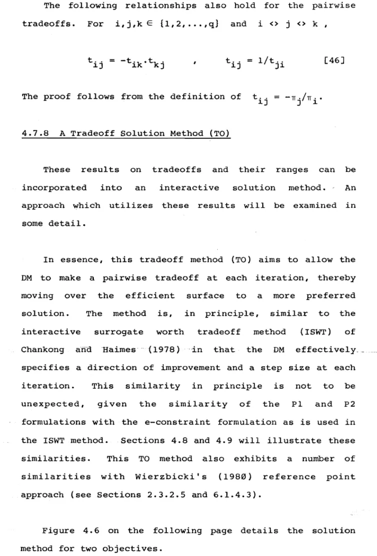
4.7.7 Tradeoffs in the Non-Linear Case 4.7.8 A Tradeoff Solution Method

4.8 COMPARISON WITH THE E-CONSTRAINT FORMULATION . . 110

4.9 A SMALL MOLP EXAMPLE • . III

4.9.1 Properly Efficient Solutions

4.9.2 Not Properly Efficient Solutions

4.10 CONCLUSION. . 121

5. A COMPARATIVE EVALUATION OF FOUR MODM

SOLUTION METHODS. . 122

5.1 THE CASE STUDY . . 124

5.2 THE SOLUTION METHODS. . 124

5.2.1 The Method of Zionts and Wa11enius 5.2.2 The Naive Method

5.2.3 The SWT Method

5.2.4 The Method of Steuer and Choo 5.2.5 Details of the Computer Code 5.2.6 Choice of Methods

5.3 EXPERIMENTAL DESIGN

5.3.1 Criteria for Measuring Performance

5.3.2 Design Considerations 5.3.3 The Experiment

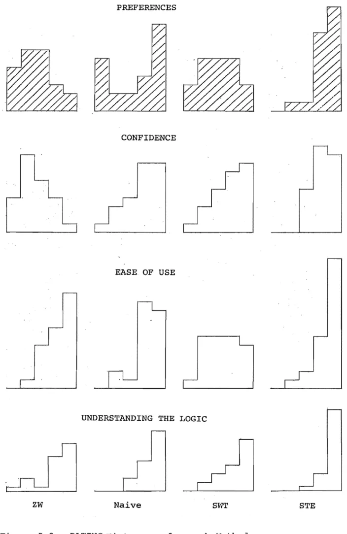
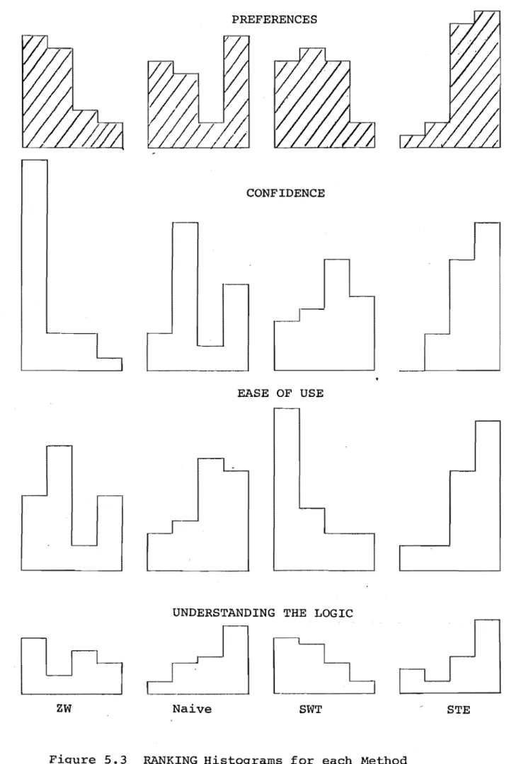
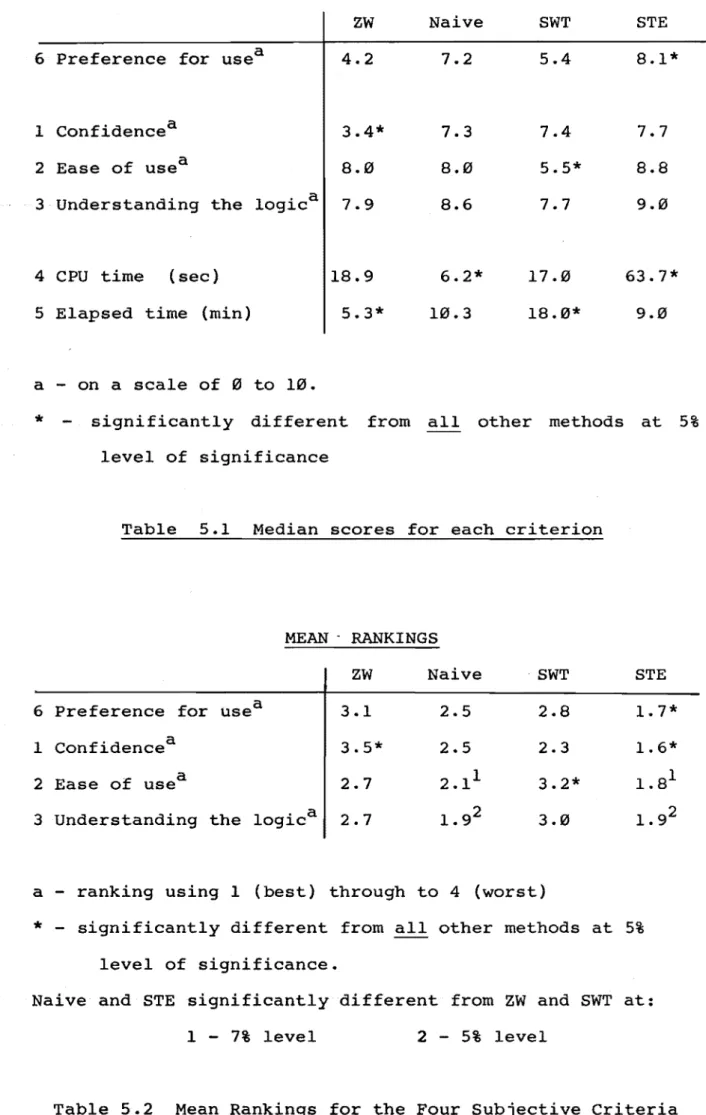
5.4 RESULTS

5.4.1 Preference for Use

5.4.2 Confidence in the Method

. 131

5.4.5 5.4.6 5.4.7 5.4.8

CPU Time Elapsed Time Additional Tests

Discussion and Implications

5.5 CONCLUSIONS.

6. THE TRADEOFF METHOD AND THE SJT METHOD

6.1 THE TRADEOFF METHOD

6.1.1 Motivation

6.1.2 Methodological Details 6.1.3 Example of Use

6.1.4 Discussion and Possible Extensions

· 153

· 154

· 155

6.2 THE SJT METHOD. . 176

6.2.1 Motivation

6.2.2 A Single Decision Maker 6.2.3 Multiple Decision Makers

6.3 CONCLUSION . 193

7. REDUCING THE NUMBER OF OBJECTIVES. . 194

7.1 LITERATURE . 196

7.2 DATA SOURCE. • 198

7.3 APPROACHES FOR REDUCING OBJECTIVE DIMENSIONALITY. . 199

7.3.1 The Statistical Measure

7.3.2 The Entropy Measure

7.3.3 Dimension Reducing Approaches

7.4 PRACTICAL CONSIDERATIONS AND AN EXAMPLE. . 205

7.5 CONCLUSIONS. . 208

8. CONCLUSION. • 210

BIBLIOGRAPHY · 215

APPENDIX 1 . _{· 226}

APPENDIX 2 . _{· 227}

APPENDIX 3 • · 230

ABSTRACT

This thesis is concerned with an investigation of solution methods for continuous multiple objective decision models (MOOM' s) . A number of different solution methods which have appeared in the

emphasis on the underlying

Ii terature are reviewed with an concepts of the methods. The following chapter examines the solution of MOOM' s from the other side, namely the behavioural aspects of decision making. Having gained an appreciation of exactly how people do make decisions, the intent of the thesis is twofold. Firstly, to develop new solution methods which can accommodate the decision maker (OM) in whatever his or her particular decision strategy is. And secondly, i t is to empirically examine four solution methods with respect to users' preferences among them. Of these four solution methods, three are among the most well known in the literature and all can cite practical application.

ACKNOWLEDGEMENTS

There are many people to acknowledge. Firstly my wife

Wendy, who has supported and encouraged me, listened and, at

times, has made me take a break from study. Also, I want to

thank my supervisor Hans Daellenbach for support and

especially for being available whenever needed. The staff

(and also my friends) of the Operations Research part of the

department,

Read were

Fred Baird, John George, Don McNickle and Grant

often used as sounding boards for ideas and

provided valuable comments. I have also appreciated the

company of and feedback from my fellow PhD students John

Giffin and Bill Baker.

I am grateful to the University Grants Committee who have

provided financial assistance in the form of a Postgraduate

Scholarship. The facilities provided by the Department of

Economics and OR for study were excellent. I want to thank

Steve Knight for assistance with the daisy wheel printer and

the Accountancy Department for letting me use it. Thanks are

also due to all those who participated in the experiment of

Chapter 5, for without them, I would have no results.

Professor A. C. Rayner and Dr G. Wood provided some helpful

comments on Chapter 7. Also, I am indebted to Fred

Martinson as i t was his PhD thesis and lectures which

provided the starting point of this thesis. Finally I thank

God, by whose grace this thesis has been seen through to

completion.

The responsibility for any typing errors and omissions

CHAPTER 1 INTRODUCTION

Man will always be faced with the need to make decisions,

decisions which must be made in the midst of a complex

environment. And most of these decisions will have

mul tidimensional consequences i i. e. , a number of different

criteria will be simultaneously affected by the decision.

Although decisions and their outcomes are necessarily quite

complex, the actual decision making process is quite simple,

and can be stated as follows.

1. There is a decision maker (DM) who seeks to achieve some

goals.

2. The DM has to choose from among two or more alternative

courses of action.

3. There is some "doubt" (in terms of goal achievement) as

to which alternative is most preferred.

This doubt on the part of the DM will inevitably occur

as he or she is faced with relevant, yet conflicting, goals

or objectives. Consider ~ decision whether to work overtime

tonight. A number of objectives are relevant: extra income,

loss of leisure, goodwill (i.e., will the boss offer overtime

again if I refuse?) and possible effects on the family

relationship_ Somehow the human DM evaluates this

information and chooses a course of action. Almost always

there will be more than just a single objective (or

criterionl ) to be considered.

1. The term "objective" will be consistently used throughout

instead of "criterion". Both terms are found in the

In the early days of management science, and especially

with regard to practical applications, the multiple objective

nature of decision problems was largely avoided. Instead,

predominantly single objective models were used, with the

most common unit of measurement being dollar value. This

single objective approach, usually in the context of a linear

programming model, resulted in a large number of successful

practical applications, which in turn stimulated greater

research in this area. The early growth of single objective

decision models is likely to have slowed developments in the

area of multiple objective decision models (MODM).

Starr and Zeleny (1977) give a brief outline of the

origins of MODM in the field of management science. This

work began in the early 1950's. After initial contributions,

the next major contribution was that of goal programming

[Charnes and Cooper (1961)]. In goal programming, a

multiplicity of objectives are reduced to a single objective

by minimizing deviations of each objective from certain

pre-specified target levels or goals. The following decade

saw traditional utility extended to multiattribute utility

theory, and with Johnsen's (1968) study on the multigoal

nature of the firm, Starr and Zeleny (p.12) suggest that

"multiple criteria decision making was firmly on its path."

A relative explosion in research, papers and applications

has occurred from the early seventies. A significant

contribution of mUltiple objective solution methodologies has

been to require more active participation on the part of the

DM in the process of determining acceptable solutions to the

MODM. This change restores in part the imbalance which

objective models in the sixties, where very little DM

participation was required.

Initially, most work on MODM presupposed an "ideal" DM

who always acted according to his or her utility function. A

number of solution methods could therefore demonstrate

convergence to the solution of maximum utility and were often

quite elegant in concept. More recently, however, a number

of researchers have sought to develop solution methods which

are more consistent with the actual decision making behaviour

of a DM and which place less emphasis on the more traditional

utility approach.

This thesis is concerned primarily with this later

development. The MODM to be considered is where the decision

alternatives are stated explicitly in the form of

constraints, with special attention given to the linear

decision model. Briefly, the thesis is structured as

follows. Chapter 2 first discusses necessary terminology and

then reviews a number of solution methodologies which have

appeared in the literature. Chapter 3 examines some features

of actual decision making behaviour and considers the

implications of these for solution methods. In Chapter 4 the

theory of a particular form of MODM is developed I which

provides a basis for new solution methods. Chapter 5 details

an experiment where four different solution methods are

compared. The experiment is designed to give a measure of

discriminatory assessment among the four methods, and also to

compare the results with the conclusions of Chapter 3. In

Chapter 6 the details of two new solution methods are given,

along with an example.

the thesis. Chapter 7

This concludes the main portion of

reducing the number of objectives in a MODM. the conclusion.

CHAPTER 2 MULTIPLE OBJECTIVE DECISION MAKING:

INTRODUCTION AND REVIEW

2.0 INTRODUCTION

This chapter is concerned with introducing necessary

terminology and definitions for the mUltiple objective

decision model (MODM). Using these definitions a number of

solution methods for the MODM which have appeared in the

literature will then be reviewed, with an emphasis on the

underlying concepts of the methods rather than on precise

mathematical detail. The first section will be concerned

only with the single decision maker (DM) situation. The

chapter concludes with a brief overview of group decision

making and a synthesis of the methods reviewed.

It is the intention of this chapter to communicate the

developments in MODM I sand . methods of solution, along with

sufficient detail, in order to provide a foundation for the

chapters to follow. Greater attention will be given to

solution methods which will be used in the experiment of

Chapter 5 and also to those which provide insight into the

developments of later chapters.

2.1 DEFINITIONS AND TERMINOLOGY - THE MODM

The MODM can be stated mathematically in terms of

continuous decision variables. The general form of the model

is

where

x is an n-dimensional Euclidean vector, x

=

l ,x2' •.. xn)

X is the set of feasible decisions

X = {x : 1! E Rn

F(1!) is a vector of scalar valued objective functions

defined on x

and "MAX" is defined in section 2.1.1 below.

The set of feasible solutions to [lJ is described by m

continuous functions of the decision variables. This is in

contrast to multiple attribute decision making (as i t is

often referred to in the literature), where the set of

feasible solutions consists of a countably small number of

discrete alternatives. The location decision for the Mexico

city Airport [de Neufville and Keeney (1972)J, and Rietveld's

(1980) study of eight development alternatives for the

Maasvlakte area in the Netherlands,are both examples where a

few well defined alternatives constitute the entire feasible

set. Approaches for solving the multiple attribute decision

problem differ considerably from those developed to solve the

continuous MODM, and will' not be discussed in this chapter.

Hwang and Yoon (1981) provide a useful survey of solution

methods for multiple attribute decision models.

2.1.1 A Definition of "MAX"

The existence of a unique optimal solution to [1] is

unlikely, except in the trivial case where a solution

x

maximizes each and every obJ' ecti ve f ( ) _{k 1 ! ,} k

= , , ...

Since such a solution cannot usually be found, the term "MAX"

does not retain its traditional meaning [Rosenthal (1982)J.

F (.!2) is not simply "greater than", ul ess than II or If equal

to", since comparisons are required to be made across

different and often incommensurable objectives. (For if the

objectives were commensurable, then [lJ could be reduced to a

single objective problem. This is the approach adopted by

traditional cost benefit analysis where i t is assumed that

all relevant costs and benefits can be expressed in monetary

terms. ) The solution to the MODM is therefore a set of

solutions, which are called efficient or non - dominated

solutions.

2.1.2 Dominance and Efficient Solutions

A definition of dominance is given below.

for (~1, x2 ) E X xl dominates x 2 if

fj(~2) < fj(xl) for some j E {I,2, ... ,q}

fk(~2) < fk(~l) for all k <> j [2J

The efficient or non- dominated set consists of all

feasible solutions to [1 J which are not dominated by any

other feasible solutions in X. Let N E X be the set of

efficient solutions. Then for any

x

to move to another

x

objective function value. Geoffrion (1968) has extended this

definition of [2J to a "properly efficient SOlution", which

requires that the marginal gain for anyone objective must be

bounded relative to marginal losses in the other objectives.

Considerable research effort has been directed to finding

solution methods which ensure that only efficient solutions

the actual optimization involves nothing more than

distinguishing between efficient and inefficient solutions.

As will be seen from the literature review to follow, almost

all MODM solution methods only consider efficient solutions;

consequently the characterization of efficient solutions is

of high priority. Kuhn and Tucker, in presenting necessary

and sufficient conditions for solving the single objective

optimization problem, also extended their work to the

mul tiple objective case. Let 1T i' i

=

Lagrange multipliers for each constraint of X and assume that

the objective functions are concave and the feasible set X is

convex. The necessary and sufficient conditions for x* E X

to be efficient are

1T . g . (x*)

=

=

~ ~

-g m

L wkgrad{fk{x*» - E 1T.grad (g. (x*» = to [3J

k=l - i=l ~ ~

-w_k ~ to , k

=

An insightful derivation of these conditions can be found in

Goicoechea et a1. (1982, pp.44-45) following an approach of

Zadeh. While [3] gives the necessary conditions for a point

to be efficient, a much more useful characterization has been

given by Soland (1979).

Let h be any function defined on Rq which is strictly

increasing on any of its components. For b E Rq define

P(h,b) = Max h[F(~)]

s.t. ~ E X [4]

If x* is an optimal solution to P(h,b), then x* is efficient.

This characterization effectively encapsulates two of the

major approaches for solving the MODM. The first is to

optimize a composite objective function (usually an additive

form) subject to the constraint set, while the second

optimizes a single objective subject to constraints on t:,he

achievement of all other objectives. These two forms are

detailed below.

q

Max L wkf_k (.!) k=l

s . t . x E X [5J

w

k ~ 0, k

=

Max f. (x)

J

-s . t . fk(x) ~ b_k ' k

=

Using Soland I s characterization a single efficient solution

can be generated by assigning values to the parameters w

k

and b k .

Alternatively, the MODM can be solved to find all

efficient solutions: this is known as the vector maximum

approach. However, since the efficient set contains an

infinity of solutions, some clarification is necessary. The

vector maximum approach has been developed for the situation

where all constraints and objectives to [lJ are linear, and

i t finds all efficient extreme point solutions (which are

finite in number). I t is then possible to describe the

infinity of non - extreme efficient solutions in terms of

2.1.3 Matrix of Extreme solutions and the Ideal Point

The matrix of extreme solutions is given by

fl(.!i> f₂(.!i) flC.!i> f₂(xi)

P = [7]

f (x*) q -q

where ~k is the optimal solution to

Max f

k (.!) s.t. x E X

The ideal solution U = (U

l ,u2, ••• ,Uq)

= (f

l (x- l*),f2(x- 2*), ... ,f (x*» q - q [8J

is given by the diagonal of P and represents the maximum

possible achievement of each objective The ideal

solution is often used as a point of reference in MODM

solution methods, where a distance measure is presented to

the DM to indicate how "far" the current solution is from the

ideal solution.

2.1.4 Decision Space and Objective Space

In MODM, a distinction is often made between decision

space and objective space. Each solution X E X can be

represented in terms of the decision variables ( x =

(X

l ,X2, ..• ,Xq) ) or in terms of the objective function values of those variables

objective space since i t is, for almost any realistic MODM,

of much lesser dimension than decision space and therefore

the presented information can be more easily assimilated by

the DM.

2.1.5 Tradeoffs

Tradeoffs are a commonly used ·concept in MODM and in

essence they are the relative changes in objectives when

moving from one feasible solution to another, i.e., they are

a measure of the difference between two solutions in

objective space. Haimes and Chankong (1979) make the

following useful distinction. Consider two feasible

solutions Define T

k . (x o

, x*)

J - - as the ratio of

change in fk to change in f

j . Thus

Then

And

T

kj is

f (xo)

=

-a p-airwise tr-adeoff if -all

f (x*) , p

=

-is a total tradeoff if

[9]

there exists at least one p such that f (xo) <> f (x*) .

p - p

-Tradeoffs can also be expressed in terms of a direction

of movement. Let d* = xO - x* be the direction in moving

from x* to and be the distance moved in that

direction, xO

=

·x* along d* can be defined as

tk . (x*, d*)

J - -

=

-=

=

=

Some methods for solving [1] seek to choose a direction d* such that only partial or pairwise tradeoffs are used, while others utilize the concept of the total tradeoff. This concept of sacrificing an amount of one objective to achieve more of another is central to MODM, especially with respect to interacti ve sol ution methods. (This concept is not as useful for multiple attribute decision problems because the tradeoffsare not continuous, but discrete.)

2.2 DEFINITIONS AND TERMINOLOGY - THE DM's PREFERENCES

Up to this point, no mention has been made of the role of the DM in finding a solution to the MODM. In the absence of any participation from the DM, the actual solution to the MODM is not a single solution, but rather a set of solutions. A value judgement (i.e., subjective information) is required

from the DM before a single "best" solution can be found. For the case of a single DM, the MODM can be restated as

II find an x* E X such that the most preferred values of

F(.!*) are obtained."

Such a solution is subjective, depending on the relative preferences of theDM among the different objectives. This is in contrast to the single objective decision model where the single best solution can be found in the absence of any sUbjective information from the DM. (Excepting, of course, where there exist alternative optimal solutions).

deviations from the ideal solution could be used. However,

since the intent of MOOM solution methods is to find the most

preferred solution, i t is unlikely that any method which does

account for the OM's preferences will achieve this.

2.2.1 utility or Value Functions

Given the inherent (and necessary) subjectivity in the

process of finding a most preferred solution, the nature of

the OM's preferences has a large impact on both the method of

solution and the actual solution values. According to

classical economics, the preferences of a rational OM are

those of a utility maximizer; i. e., a DM is able to search

among the set of feasible solutions and choose that solution

which provides the greatest satisfaction or utility. utility

theory therefore assumes that, for an individual DM, there

exists a scalar measure of preference for each x E X which

is his or her utility function.

There are certain conditions which the OM I S preferences

must satisfy for a utility function to be defined on them.

The DM must be able to express both consistent preferences ..

and consistent beliefs, and these beliefs (what the OM thinks

is going to happen) are to be independent of preferences

(what the OM would like to happen) [Hogarth (1980, Chapter

4)J. Consistent pref~rences imply transitivity; i.e., if A

is preferred to Band B to C, then A is preferred to C.

Consistent beliefs imply that predictive judgements regarding

the occurrence of events can be formulated as probabilities,

which means that there exist lotteries for which certainty

equivalents can be derived, e.g., Keeney and Raiffa (1976,

Let V [F(~)] be a utility function which represents the

preferences of a DM (as scalar values) over the set of

feasible solutions. The MODM can be reformulated to find the

most preferred solution by solving

s.t. x E X _[llJ

In [11] all objectives have been aggregated into a single

scalar measure which is then optimized to find the solution

x* of maximum utility. The practical difficuLty with this

approach is the determination of a suitable form for V.

In order to facilitate the assessment of the overall

utility function V

,

i.

e.,

V [fl(~),f2(~), ..• ,fq(~)J

= H(V_l [f_l (x},V₂[f

2(x)], ...

,v

- - q q - [12]

A simple and commonly used form for H is the weighted

additive form, which for three objectives can be stated as

V[fl(~),f2(~),f3(x)J

= wlVl[fl(~)] + _{w2V2 [f2 (x)]} + w3V3[f3(~)J [13J

where wk ' k =1, 2 I 3 measures ~he relative contribution of

each objective. Zeleny (1982, p.4l8) lists some other common

decomposition forms. The "cost" of using decomposition forms

is that a further two conditions are placed on the DM IS

preference structure. These are preferential independence,

where the value of a tradeoff between any two objectives is

independence where the DM's preferences for lotteries on one

objective are independent of the level of a second objective.

In practice, i t is assumed that these conditions hold,

because unless some simple decomposition form is used,

assessment of the DM's utility function is almost impossible.

2.2.2 Marginal Rate of Substitution

In contrast to the tradeoffs previously mentioned in

Section 2.1.5, the marginal rate of sUbstitution (MRS) is the

value of a tradeoff caccording to a DM's utility function,

rather than according to the geometry of the feasible set

x.

The MRS is a pairwise tradeoff, not a total tradeoff. With

respect to a utility function V, MRS

kj is defined as the

amount of fk that a DM is willing to sacrifice to acquire

an additional unit of f.

J at any given point

objective space, i.e.,

MRSkj(fO)

=

j )

I

= -

j for fixed utility.

in

[14J

Figure 2.1 on the following page shows both tradeoff and

MRS values. This figure shows the set of feasible solutions

in objective space (only two objectives) with the DM's

utility function superimposed on top for certain fixed levels

of utility. The efficient set is defined by the line

segments

Be

=

B 6

4

2

/ d i r e c t i o n of improving

utility

V=20

V=lS.

set of feasible solutions in objective space

--I

~--~--~~--~-~--~---B+=~~-~~----!~

f1

Figure 2.1

At 0

=

At G MRS

21 = 2.83 and

This MRS value indicates that, at solution G, the DM is

willing to sacrifice up to 2.83 units of to gain an

additional unit of f

l , whereas the tradeoff value at G says

that an additional unit of can be obtained by

sacrificing only 0.25 units of There are obviously

better solutions than G.

2.2.3 Monotonicity of Preferences

A further assumption which is usually made in the context

of the MOOM is that the OM's preferences are a monotone

assumed to always prefer more to less: his or her

satisfaction does not decrease as fk ' k E {1,2, .•. ,ql

increases. The marginal value of an extra unit of objective

fk ' k E { 1 , 2, ..• , q

1

The consequence of this assumption is that the OM's most

preferred solution will always be efficient. This assumption

also accounts for the large emphasis which has been placed on

generating efficient solutions to the MOOM [1]. In general,

the monotonicity of preferences assumption is a reasonable

one, especially when care is taken to appropriately define

the objectives. As a contrary example, consider an objective

in a financial MOOM which is to achieve a current ratio with

a value of 2. For this objective I a OM's preferences are

likely to be represented by the curve in Figure 2.2 below.

Maximization of the current ratio is an inappropriate

objective; a more realistic objective for which preferences

are monotone would be to minimize deviations from the ideal

value of 2.

preference

2

Figure 2.2

This concludes the introductory terminology and

definitions as relevant to the MODM and necessary for the

following discussion.

2.3 METHODS OF SOLUTION

Some of the solution methods for MODM's which have

appeared in the literature will now be discussed. For other

more detailed reviews see Hwang and Masud (1979) or Chankong

and Haimes (1983a).

Multiple objective solution methods vary according to the

characteristics of the problem formulation (e.g., linear or

non - linear and size) and according to the information

provided by the DM. Hwang and Masud (1979) provide a useful

classification of methods according to the timing of the

information provided. Their three categories are

a priori before solution

progressively during solution (interactive methods)

a posteriori after solution.

A different approach is taken by Ho (1981) who proposes a

hierarchical classification according to the quantity of

information provided. This section will follow the

classification of Hwang and Masud and consider only the ,

single DM situation. Also the emphasis will mainly be on the

linear MODM, as this has been the focus of most research.

The review of solution methods will not consider any methods

in great detaili rather i t is intended to present underlying

concepts of the major solution methods. This is to

demonstrate the various solution approaches and also to

provide sufficient background for the discussion of the

2.3.1 A PRIORI ARTICULATION OF PREFERENCES

The solution methods in this category first elicit

subjective information from the DM which is then utilized to

find a preferred solution.

2.3.1.1 Goal programming

Before the advent of multiple objective solution methods,

the method of solution usually consisted of maximizing a

single objective with all other objectives constrained to

certain acceptable or satisfactory levels. Goal programming

(GP) was the first truly multiple objective solution method

to be developed [Charnes and Cooper (1961)], and is based

around the intuitive concept of goal setting. Specifically,

the DM assigns a goal or target to each objective and then

seeks to minimize the deviations from each goal. These

deviations, which represent both over and under achievement

of goals, are then weighted ~y the DM so as to reflect their

relative importance. The GP formulation of [1] is

q

Min E (W;d; +

w~d~

k=l

s.t.

fk(~)

d~

x E X

d; , d;

,

,

k=1,2, ••• ,q

[lSJ

where G_k is the goal for objective k and d; and d; are

measures of over and under achievement respectively.

The deviational weights and can be either

pre-emptive, in which case goals of higher priority must be

or additive, whereby all goals are at the same priority level

and considered simultaneously. Combinations of these two

cases are also possible, e.g., using additive weights among

three objectives which all have the same priority. The

informational burden placed on the OM is to specify two types

of information for each objective before solution. These are

the goals G

k to be attained and the weights wk'

A number of similarities can be seen between GP and the

first high level computer language, FORTRAN. Both represent

pioneering efforts in a particular area and have now become

well established and widely used. In the same way that, as

more computer languages have been developed, FORTRAN (in its

original form) has come under much criticism, goal

programming has also faced not inconsiderable criticism. This

criticism includes the substantial burden placed on the OM to

provide realistic goals before solution, the possibility of

generating inefficient solutions [Zeleny (1982, pp.296-298)]

and the validity of tradeoffs under a pre-emptive weighting

structure. As Rosenthal (1983) points out, the use of

pre-emptive or priority weights is contrary to the concept of

a MRS. pre-emptive weights imply that since one objective f.

J

must be fully satisfied before a second objective is

even considered, the is infinite. No amount of

inducement will convince the OM to sacrifice some of f. to

J

gain some of f

k; a result which is contrary to intuition.

However, when compared with other MOOM solution methods,

GP can attest to a wealth of applications, [e.g., Lin

(1980)] . While this is in part due to its position as a

pioneering solution method, the widespread use of GP can also

of setting goals and trying to get as close as possible to

them. Furthermore, GP can accommodate certain decision

situations which are more difficult with other solution

methods. For example, Sartoris and Spruill (l974) use GP in a

financial decision model where objectives are not always

linear and preferences are not monotonic for given

objectives. In their working capital model one objective is

to achieve a liquidity ratio of one,

i. e. , ( xa + 40x₂ + 52.5x₄ ) / ( 150 + x₇ )

=

This can be multiplied through and deviational variables

added to give

- +

xa + _40x2 + _{52.5x4 - x7} + d - d

=

where minimization of the deviations will seek to achieve the

desired liquidity ratio. An alternative solution approach

would be to use fractional objectives [e.g., Choo and Atkins

(1980)J.

Unlike many other MOOM solution methods which attempt to

converge to the OM t s most preferred solution, GP is more a

mechanism for generating solutions which will reflect the

goals and weights specified by the OM. Consequently, there

is no guarantee with GP that the most preferred solution will

be found.

It is not surprising to find that GP methods have been

extended to interact with the OM in order to relieve some of

the burden of a priori information provision and to provide a

more systematic approach in searching for the most preferred

2.3.1.2 Surrogate Worth Tradeoff (SWT) Method

This method is based on the previously mentioned

characterization of an efficient solution [6J, which is known

as the e-constraint formulation. It is

Max

s.t. fk(x) ~ e_k ' k

=

x E X .

[16J

Developed by Haimes and Hall (1974), SWT utilizes the

concept of a pairwise tradeoff between two objectives. It

can be shown that for F differentiable and _{" jk being the}

Lagrange multiplier for constrained objective k, the pairwise

tradeoff is defined as

[17J

In the SWT method the DM is required to assign a value to

various pairwise tradeoffs which are presented to him or her.

Specifically, for different efficient solutions the DM

assigns a value w ..

1 ) to each pairwise tradeoff >. .. 1) for

i,j E {1,2, ..• ,q}. The preferred solution will be where

w ..

=

1) for all i , j

,

e.,

Using the following relationships,

" .. = ₁₎

1/" ..

,

all pairwise tradeoffs can be calculated for any properly

efficient solution to [16J. (At any improperly efficient

solution, some >.'" i E{1,2, .. ,q}, i <> j

1) will be zero.)

w.. are called the surrogate worth functions and are ordinal

1)

in nature. If w .. > 0 then i t is assumed that MRS .. > >. ..

(the tradeoff is favoured, i.e., decrease f. and increase

1.

f . ) . For w.. < '" , the reverse applies. After the DM has

J 1.J

provided this information at a number of solutions, a solution in objective space is determined whereby _{w ..}

= '"

1.J

for i

=

J This solution will then be

the most preferred solution, where the DM has provided these worth assessments prior to solution.

often i t is not specified exactly how the indifference solution(where all w. ,'s

1.J are zero} is calculated. If in the

course of the evaluation, one such indifference solution is found, then there are no difficulties. However this is generally not the case. When there is no point of indifference immediately obvious from the w ..

1.J values, the

most commonly recommended approach is to use multiple regression. q-l regressions-are performed of the form

w

kj = wk ( f 1 ' f 2' ... , f q ) for each k E {1,2, ... ,q}, k <> j where w

kj are the worth assessments for the pairwise tradeoff between _fk and f ..

J setting all the wkj =

'"

gives a set of q-l simultaneous equations which can be solved to find the indifference solution with values

( fi ' fi ' ... , f~) These values are substituted into [16J which is then solved to find f~. On the basis of a small

J

According to Haimes et al.(l975, p.34), the SWT method is

based on the fact that "optimization theory is usually more

concerned with the relative value of additional increments of

the various non-commensurable objectives, at a given value of

each objective function, than i t is with their absolute

values" . This, coupled with the observation that i t is

generally easier for a DM to provide pairwise tradeoffs than

total tradeoffs, provides the motivation for the method.

As GP methods have been made interactive, so too has the

SWT method. Chankong and Haimes (l9~8) describe the

interactive surrogate worth (ISWT) method which will also be

mentioned in section 2.3.2.2.3 •

GP and the SWT method, along with utility function

\

assessment, are the main solution methods where information

is provided by the DM prior to solution. The extension of

these two methods to an interactive form is likely to be

indicative of the unsuita~ility of a priori information

provision.

2.3.2 PROGRESSIVE ARTICULATION OF PREFERENCES

The majority of MODM solution methods belong in this

second category. The intent of these methods is that via

interaction and progressive revelation of preferences, a

sequence of solutions will result. This sequence of

solutions should in the limit converge to the most preferred

2.3.2.1 STEM Method

The STEM method, proposed by Benayoun and his colleagues

(1971) for linear MOOM's, was one of the first interactive

solution methods to be developed. It is conceptually simple,

with the preferences of the OM being implicitly incorporated

into the solution method by setting bounds on the objectives.

The formulation combines [6J with a variation of [5J with the

OM being required to progressively provide values for b.

The parameters of the function h are determined

endogenously and are a form of weighted distance metric from

the ideal solution. At the first iteration the following

problem is solved.

Min y

s.t. Y > _{(Uk-fk(x})wk ' k} = 1,2, .•. ,q x E X

[19J

where Uk and w

k are calculated from the extreme solution

matrix. The Uk values are £ound from the diagonal elements

and the w

k values are calculated as

q

=

k=l

Mk is the minimum value of each column k of the extreme

solution matrix and c_jk are the coefficients of each linear

n

objective function, fk <..~)

=

j=l J J

interpreted as a measure of the relative discrepancy between

the maximum and minimum values of fk(x}. A solution x to

[19J is presented to the OM in terms of the objectives. The

OM is then required to specify an amount by which a

satisfactory objective fj is to be relaxed in order to allow

iteration, the constraint set is augmented by a constraint of

the form

f.{x) > f.(i) - O.

J - J - J [21]

where

o .

J is the amount of relaxation. w. is then set to J

zero and the next iteration begins. Since the DM sets bounds

for a different satisfactory objective at each iteration, the

procedure should terminate after q-l iterations with either

the most preferred solution or the message that there is no

solution acceptable to the DM.

A number of extensions to this approach have been

proposed. These include Belenson and Kapur (1973) who use a

two person zero sum game approach to determine the

appropriate weights at each iteration, and a goal programming

extension of the STEM method [Fichefet (1974)]. Nijkamp and

Rietveld (1976) suggest that the weights at each iteration

can be chosen such that each. solution of the extreme solution

matrix is valued equally. In matrix notation, the

appropriate weights are

[22 ]

provided the extreme solution matrix P is non- singular. A

disadvantage with this approach is that negative weights may

be generated. And because Nijkamp and Rietveld use an

objective of the form w.C (where C is the matrix of

objective function coefficients), the use of negative weights

may result in inefficient solutions being generated at some

2.3.2.2 Method of Geoffrion, Dyer and Feinberg (GDF) (1972)

In contrast to the STEM method, the GDF method places a greater informational burden on the DM, in that he or she is required at each iteration to provide a MRS value for any pair of objectives. The method assumes that, at least implici tly, the DM possesses a utility function defined on the q objective functions. The MODM therefore becomes that of [11]

i . e. I Max V [F(x)]

s.t. x E X . ' [23]

[23] is solved by utilizing the Frank-Wolfe algorithm,

which itself uses linear approximations to the utility function at each iteration. There are two steps at each iteration: finding a best direction of improvement and finding a best step size in that direction. At a feasible (although not necessarily efficient) solution the direction finding problem for [23] reduces to

s.t. : l E X [24J

where wk(xi )

=

j • The neat thing about this method is that the exact form of the DM • s utility function is not required. Provided that the DM is able to give MRS information at each iteration, which is consistent with his or her utility function, the direction of best improvement di can be found. In order to find the step size a, various values of

are presented to the OM, who chooses the most preferred one. The next feasible solution

iterations continue.

'+1

x~ _{is found and the}

The sequence of solutions which can begin at any feasible solution, will not necessarily be efficient until the final, most preferred solution is reached. As . regards possible disadvantages of the method, Hwang and Masud (1979, p.121) comment that the OM often has difficulty in providing MRS information at each iteration and where there are more than two objectives, the choice of a suitable reference objective can also be difficult.

A number of other solution methods which are similar in spirit to the GOF approach and yet exhibit further extensions in concept will also be briefly reviewed.

2.3.2.2.1 Efficiency Projections - Winkels and Meika (1984)

This approach generates only efficient points at each iteration. Once the direction of best improvement has been found from the MRS information of the OM, i t is projected onto the efficient surface. This information is presented graphically to the OM who then chooses the appropriate step size. Figure 2.3 (on the following page) which is taken from the article, gives an example of the efficiency projections for a single iteration. If the ordinary linear approximation of the GOF method is used, the result is a straight line between the endpoints of A

=

=

information is presented provides considerable insight into the total tradeoffs in a given direction.

The method is exactly that of the GOF method, except that the initial and all sUbsequent solutions are efficient.

~ ~ ::; ~

I

;

l!! ~

s

fJ

~

:9 I:? ~ Iii!

~

5

w <:

II'> .... .., co cr:

.... w ....

...

::::

;-1

;~

Ut<il

u::r

~~ 2:

~!i=l .... _~!li .... -,

-

.

I!-(

0 0 0

~

-'

""

0

""

,1

-

~ fil .,..

-

1

I

J

!':! i F;i

.

'i ..t .!!

A

* Objective 1 _{~ Objective 4}

.;. Objective 2 _{& Objective 5}

*

Figure 2.3

2.3.2.2.2 Proxy Approach - Oppenheimer (1978)

local approximation to the OM's true utility function than a

linear approximation as used by GOF. The proxy utility

functions are not intended to be globally valid: in fact a

different proxy will be evaluated at each iteration. Two

standard form proxy utility functions used by Oppenheimer are

q

sum-of-exponentials: V[F] = - k:l ~exp(-wkfk)

sum-of-powers : V[F]

[26]

The choice as to which form of proxy funotion is actually

used is at the discretion of the analyst. This proxy

approach has a considerable advantage over the GDF method

since both the best direction of improvement and the step

size are calculated from the local proxy utility function at

each iteration.

2.3.2.2.3 SPOT Method - Sakawa (1982)

It is necessary to briefly introduce the interactive

surrogate worth tradeoff (ISWT) method [Chankong and Haimes

(1978)J in order to illustrate the SPOT method. The ISWT

method is an interactive scheme based on the e-constraint

formulation [16J. It uses zoutendijk' s method of steepest

descent to determine a direction of improvement, which is

found from the worth values provided by the DM, and a step

size at each iteration. At a given solution x , surrogate i

worth values are assigned by the OM to each tradeoff

Ajk The updated right hand side of each constrained

objective k is simply given by

where {l is the step size. The similiari ty with the GDF

method can be easily seen; the values contain the

necessary MRS information. This procedure will converge to

the most preferred solution under the assumption of an ideal

DM (who conforms to his or her implicit utility function).

·The SPOT method· uses the same basic approach as the ISWT

method except that (like Oppenheimer) a proxy utility

function is used to determine the best direction of

improvement. specifically, if is the MRS_jk based on

the DM' s proxy utility function at solution x , then the i

updating equation is

[28J

Both SPOT and Oppenheimer's proxy approach require

consistency checks to be made of the DM' s preferences with

regard to the particular proxy function which is being

assessed. If discrepancies exist beyond a certain

prespecified tolerance level, the inconsistency is explained

to the DM so that the tradeoffs can be reassessed and the

discrepancy resolved.

Sakawa and Seo (1983) have further extended the SPOT

method by using fuzzy set theory. They assume that the DM

has a local, but imprecise knowledge of his or her utility

function. This means that instead of having to specify an

exact value for each MRS assessed, one approach is to require

the DMto provide four values. These four values are the

absolute minimum and maximum for the MRS and the minimum and

maximum of a totally acceptable interval for the MRS. This

numbers. Here an attempt is made to accommodate some of the

imprecision expected from a OM, and therefore there must also

be some tolerance of inconsistency.

2.3.2.2.4 Tchebycheff Norm Approach - Sakawa and Mori (1983)

Instead of using the e-constraint formulation as in the

SPOT method, in this method Sakawa and Mori use a weighted

Tchebycheff norm formulation. (This Tchebycheff formulation

will be discussed in considerable detail in Chapter 4.) A

direction of improvement d is found using MRS information

provided by the OM. Wi th a step size parameter of A ,

solutions in this direction (f( x*) + A d) are then found I

except that these solutions are first transformed into

efficient solutions by using the Tchebycheff formulation.

This approach is similar in principle to that of Winkels and

Meika (1984) where all solutions in the direction of

improvement are projected onto the efficient surface. The

difference lies with the actual projection mechanism.

This section has reviewed a number of extensions to the

original GOF method. Given all these variations, there is

the potential to combine some of these approaches to arrive

at a useful solution methodology.

2.3.2.3 Method of Zionts and Wallenius (ZW) (1976,1982)

In order for this method to be of practical use for

solving the MOOM (lJ, i t is required that all functions be

linear. Furthermore i t is assumed that the OM's underlying or

implicit utility function is a linear combination of the

Max

q

V = k:l wkfk(x) s.t. x E X

q

L w

=

[29J

,

At each iteration a set of weights w

=

l ,w2' ... ,wq) is determined until the process terminates with the weighting

structure which maximizes the linear utility function. The

most preferred solution will be an extreme point of the

efficient set because the composite objective in [29J is

linear. Specifically, the method operates as follows. An

arbitrary set of weights which satisfy [30J are chosen

(usually equal weights in the absence of other information)

and the resulting solution xP is found. Then for each

non-basic variable the following subproblem test is

performed.

q

Min f _r

=

k=l

q

s.t. L v

k .wk > 0

,

.

.

k=l J

Let f: be the optimal solution to [31J. If f* < 0 then

r '

introducing x~ into the basis will result in moving along

an efficient edge to another efficient solution. Zionts and

Wallenius also implement some "quick check" rules such that

some non - basic variables are immediately eliminated from

consideration, which reduces the necessary computational

effort. The values are the Lagrange multipliers from

the optimal simplex tableau to [29J and [30J for objective k

and non-basic column j. Effectively, v.

-J

is the total tradoff vector which results

= (v 1 j , v 2 j , ... , v qj )

if x~ is pivoted

into the basis to give an adjacent efficient solution. The

DM is required to provide an ordinal response of "yes", "no"

or I' indifferent" to each total tradeoff v .•

-J

The burden placed on the DM as regards providing

information is affected in two ways. It is lessened in that

only ordinal rather than cardinal information is required,

but is increased in the sense that the DM has to aSsess the

tradeoff holistically, i . e • I over all objectives

simultaneously_ From the DM I S responses, constraints are

constructed as follows

I 'yes " :

II no" : f 3 < e « 1 [32J

with .. indifferent" responses being omitted for reasons of

accuracy and speed of convergence. A II yes .. answer implies

that the DM prefers the tradeoffs in the direction of an

adjacent solution xp+l therefore i t must have greater

utility than the old solution xp •

i .

e.,

v

=

k > e

k=l J

[33J

since

After responses to every tradeoff vector V'I a feasible

-J

set of weights w2 which satisfy [32 J are found. These

weights are used to solve [29J and [313], as the next

iteration of the method begins. A new set of tradeoffs are

presented to the DM and the process continues with each

[32J. (When subsequent subproblem tests [31J are performed

the constraint set of [32 J is also appended to ensure that

adjacent efficient extreme points, which are not consistent

wi th previous responses, will be excluded). The process

terminates when there is only one efficient extreme point

which is consistent with the previous responses of the DM.

Effecti vely, the ZW method cuts away a portion of the

objective space at each iteration, with the advantage that

many solutions can be implicitly eliminated. De Samblanckx

et al.(1982) have observed that in this method one wrong

answer is irrevocable and that tradeoffs are not always

fulfilled exactly how they are presented to the DM. Since

this method is included in the experiment of Chapter 5, some

of these issues will become clearer as an example of the

method in operation is given.

More recently, Stewart (1984) has proposed a modification

to the ZW method whereby provision is made for inconsistent

choice behaviour. The problem of finding the vector of

weights w at each iteration is approached by maximizing the

following log likelihood function.

L(W:S ) _{- n}

=

q

E log [ 1 + exp(- E wkv

kJ') J

, E S k=l

J n

[34J

where S is a set of pairwise preference statements given

n

by the DM. While there are some additional features to

Stewart's logistic regression approach, the basic concept is

to allow for inconsistencies by using maximum likelihood

estimation. However, despite Stewart's own comment that lithe

Zionts-Wallenius method is quite often relatively insensitive

represents another attempt to reduce the requirements placed

on the OM as information is progressively elicited from him

or her.

2.3.2.4 Method of Interval Criterion Weights

and its Extensions

Again i t is assumed that the MOOM is linear. This method

[Steuer (1977)J derives from methods for generating the

entire efficient set (see section 2.3.3) and 'earlier work of

Steuer (1976). In this earlier work, Steuer showed how the

size of the efficient set can be reduced if the OM is able to

a priori specify bounds on the weights as in the following

weighted sum formulation.

q

Max L _wkfk (!.) k=l

s.t. x E X [35]

-q

i:: w_{k =} 1 k=l

w_k E _(mk,u

k)

"

-

-

[35] cannot be solved in its current form; however, steuer

shows that i t can be reduced to

s.t. x E X [36]

where d j , j = 1,2, ••. , r represent the extreme rays of the

reduced gradient cone as defined by the bounds m_k and uk on

the weights. (The gradient cone or cone of "good directions"

is the convex cone generated by the gradients of the

different objectives.) Each extreme ray d_j is defined by

i .

e.,

where the critical weights are determined by feasible

combinations of the interval endpoints (mk,u

k). For a given set of interval bounds, i t is not possible to determine in

advance the number of extreme rays r required to define the

reduced gradient cone. The gradient cone can perhaps best be

visualized (in objective space) by imagining a light source

at the origin which shines on the efficient surface.

Initially the cone of light illuminates the whole surface and

i t is narrowed down as interval bounds are specified for the

weights.

It is this process of narrowing down the light cone which

steuer has developed into an interactive method. In terms of

the above illustration, the cone of light initially

illuminates the whole efficient surface. 2q+1 extreme

solutions dispersed over this illuminated area are presented

to the OM who chooses the most preferred one. The central

axis of the cone is then moved to this chosen solution and

the cone is reduced to l/qth the cross sectional volume,

thereby illuminating a proportionately smaller area around

. the chosen point. A further 2q+1 efficient extreme point

solutions are presented, and the process continues until the

OM requires the generation of all efficient extreme point

solutions within the reduced light cone. At this stage, the

set of efficient extreme point solutions should be of a

sufficiently small size to be comprehensible to the OM.

Mathematically, this procedure generates a new set of

interval bounds at each iteration, with each reduced gradient

As with the ZW method, the DM is required to make

holistic comparisons among solutions, and i t is assumed that

the DM has a linear utility function since only extreme point

solutions are ever generated. However there is no guarantee

that the method will converge even under the assumption of an

ideal DMwith a linear utility function [Z ionts (1982, pp.

4.21-4.25)].

The fact that only extreme point solutions are generated

by this method may have prompted Steuer to develop i t further

[Steuer and Choo (1983), Greis, Wood and steuer (1983)J. In

this extension a formulation that is different from the

weighted sum approach is used. It is the Tchebycheff

norm formulation and has the capability of generating every

efficient point. A large number of possible weighting

vectors are randomly generated and then "filtered" to choose

a subset of the most dissimilar vectors, where the filtering

process is based on a distance metric. The Tchebycheff

formulation is then repeatedly solved using each weighting

vector of the filtered set. The set of resulting solutions

is again filtered and the DM is presented with a small subset

of efficient solutions which will be representative of the

efficient set. Again the gradient cone is reduced around the

most preferred of these solutions and based on the resulting

set of interval

generated. As

bounds a new

the gradient

set of weighting vectors is

cone shrinks down at each

iteration, the sequence of solutions is expected to converge

to the most preferred solution; however, given the random

component in the method, a rigorous proof of convergence is

not possible. This Tchebycheff method is also included in

2.3.2.5 The Method of the Displaced Ideal and the Reference

Point Approach

The method of the displaced ideal [Zeleny (1976,1982)] is

perhaps more based on empirical studies of decision making

behaviour than the methods reviewed thus far. It is based on

the concept that choice between alternatives may differ

depending on the point of reference which is used. The

obvious choice for a point of reference is the ideal

solution, which can be displaced as some solutions are

excluded rrom the efficient set. The method, which is

interactive, is illustrated in Figure 2.4 below

for two objectives.

A ... - ... ----... - ... -l-....

--~.L

...

+--.

B ...

JG. ...