Genetic algorithm approach to the quality-related
assembly line balancing problem
Choosak Pornsing, Arnat Wattanasungsuit*
Abstract—this article describes the approach of a genetic
algorithm for solving quality–related assembly line balancing problem. The algorithm was taken into account of the requirements of how to minimize the cost of operation and maximize the resources utilization, while simultaneously maintaining the quality of assembled products. Model of genetic algorithm with random-weighted-sum combination used in this study was analyzed the existing data of sample factory showing that significantly fewer resources would be required, better line efficiency was obtained, and the quality of assembled products was also maintained compared to existing performance.
In addition, optimum genetic parameters were obtained by full-factorial experimental design.
Index Terms—Assembly Line Balancing, Design and
Experiment, Genetic Algorithm, Genetic Parameters
I. INTRODUCTION
The assembly line was first introduced by Henry Ford for producing the T-model car [1]. It has been widely applied for assembling automobiles, appliances, computers and other consumer products [2]. The goal of assembly line designed is to create a smooth, continuous flow along the assembly line with a minimum of idle time at each workstation. A well-balanced assembly line has the advantage of high personnel and facility utilization and equity among employees’ work loads. Its terminology is Assembly Line Balancing Problem (ALBP). The ALBP is how to group the assembly activities, which have to be performed in an assembly task, then, put them into workstations, so that the total assembly time required at each workstation is approximately the same [3]. The cycle time of the assembly line is determined by the workstation with maximum total assembly time. There are two versions of the problem. Assuming an identical line assembly workstations and a set of tasks to be processed, the Type I simple assembly line balancing problem (SALBP-I) consists in finding an assignment of tasks to workstations such that the required number of workstations is minimized. The problem is constrained by a set of precedence relations between the tasks and a given cycle time, corresponds to maximize work time
available per workstations. The Type II simple assembly line balancing problem (SALBP-II) consists in allocating tasks to given number of workstations in order to minimize the cycle time, i.e. the maximum work time of any workstation [4]. SALBP was specified by the following assumptions: 1) all input parameters are known with certainty, 2) a task cannot be split among two or more stations, 3) tasks cannot be processed in arbitrary sequences due to technological precedence requirements, 4) all tasks must be processed, 5) all stations are equipped and manned to process any task, 6) task time is independent of station where they are performed and of the preceding task, 7) any task can be processed at any station, 8) the line is serial, 9) the line is designed for a unique model of a single product, 10) for Type-I, the line cycle time is given and fixed and for Type-II, the number of workstation is given and fixed. The ALBP is difficult to be solved because they are involved in complex combinatorial optimization. If n tasks are to be performed on m
workstations, for instance, there are potentially (n!)m
solutions, although many of these may be infeasible due to precedence constraint and the others [5]. So, ALBP was named the NP-hard class of combinational optimization problems, which implied that some heuristic methods should be used to solve large-scale ALBP [6]. However, there are many objectives in the real-world being extended from the traditional objectives, such as need to maintain the quality of assembled products and required to have fast computational algorithms etc [7]. So, nowadays, the intuition and judgment are still used to design the assembly line, especially in a small and medium manufacturer. Accordingly, the primary of this study was to propose a multi-objective model of genetic algorithm being taken into account the quality of assembled products, improvement of the production efficiency and reduction of production cost simultaneously. The full-factorial experimental design was used to determine significant genetic parameters and their suitable level.
Manuscript received November 9, 2007. This work was supported in part by Silpakorn University.
Choosak Pornsing is a lecturer with Industrial Engineering and Management Department, Faculty of Engineering and Industrial Technology, Silpakorn University, Nakornpathom 7300, Thailand (e-mail: [email protected]).
Dr.Arnat Wattanasuangsuit is an associate professor with Industrial Engineering and Management Department, Faculty of Engineering and Industrial Technology, Silpakorn University, Nakornpathom 7300, Thailand (corresponding author, phone: +66 34 254236; fax: +66 34 254236; e-mail: [email protected]).
II. GENETIC ALGORITHM ASSEMBLY LINE BALANCING PROBLEM
Genetic algorithm (GA) is a general concept for solving complex optimization problems which is based on manipulating a population of solutions by genetic operators like selection, recombination, and mutation. It is started by encoding the problem to produce a list of genes. The genes are then randomly combined to produce a population of chromosomes, each of which represents a possible solution. Genetic operations are performed on chromosomes that are randomly selected from the population. This produces offspring. The fitness of these chromosomes is then measured and the probability of their survival is determined by their fitness. The genetic algorithms had been widely applied to assembly line balancing problem [3], [6], [7], [9]. Almost of these studies were conducted on multi-objective algorithms. Y. K. Kim et al. [6] used a GA for assembly line balancing with various objectives. Firstly, minimizing number of workstations, Secondly, minimizing cycle time, Thirdly, maximize workload smoothness, Fourthly, maximizing work relation, and Lastly, a combination of third and fourth objectives. They also proposed the repair mechanism fixing an infeasible offspring so that the offspring became feasible. This significance of the repair method was that it allowed us to employ diverse genetic operators in solving an ALB problem. The results of this study was compared to the known heuristic algorithms, Kilbridge and Wester, minimum upper bound (MIN-UB), maximum task time divided by task upper bound (MAX-DUR/UB), maximum task time (MAX-DUR), largest set rule (LSR), and Rachamadugu and Talbot’s method (R&T). It was shown that their approach had better results. S.G. Ponnambalam et al. [7] proposed a multi-objective to solve assembly line balancing problems. The performance criteria, the number of workstations, the line efficiency, and the smoothness index were the multiple objectives. In addition, they had compared the multi-objective genetic algorithm with other heuristic algorithms, ranked position weight, Kilbridge and Wester, for example. They found that GA performed better in all performance measures than the other heuristics, but the execution time of GA was longer than the others. R-S. Chen et al. [9] proposed a hybrid genetic algorithm which was taken into account minimizing cycle time, maximizing workload smoothness, minimizing the frequency of tool change, minimizing the number of tools and machines used, and minimizing the complexity of assembly sequences. The self-tuning method was also developed to enhance the effective schemata of chromosome during GA processing. As mentioned above [6], [7], [9], these studies were conducted in advance, however it did not consider the quality of assembled product being affected by the configuration of assembly line. Consequently, unique assembly line balancing genetic algorithm (ALBGA) model was developed for our sample factory as a case study.
III. GENETIC ALGORITHM FOR THE QUALITY-RELATED ASSEMBLY LINE BALANCING PROBLEM
As mentioned in the last section, the multi-objective was proposed in this research. The quality of assembled product, the cost of operation, and resource utilization were explored simultaneously. A repair process based upon precedence adjustment was used in order to rectify infeasible solution
that could be produced by genetic operations [6]. The algorithm is illustrated in Fig.1.
A. Representation and initial population
The first step in construction a genetic algorithm is defining a genetic representation (encoding). The encoding scheme being employed herein is an integer encoding which was proposed by Y. Y. Leu et al. [10]. All tasks are sequentially listed in the order that the tasks are assigned to workstations, this principle was named is Sequence-oriented representation. An initial population is randomly generated, the number of chromosomes in the initial and subsequent populations is constant and is denoted by Popsize. Next provided is a method of generating one random and feasible sequence. It is a version of topological sorting transforming a partial ordering into a linear ordering.
Step 1: form an initial available set of tasks having no predecessors, and create an empty string. Step 2: terminate, if the available set is empty. Otherwise, go to Step 3. Step 3: select a task from the available set at random, and append it to the string. Step 4: update the available set by removing the selected task and by adding every immediate successor of the task if all the immediate predecessors of the successor are already in the string. Go to the second.
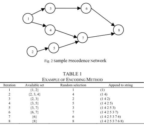
[image:2.595.336.538.419.541.2]Note that in Step 4 the available set is updated with tasks satisfying precedence constraints so that it always ensures the generation of a feasible sequence. Fig. 2 is a sample precedence network being used to depict the encoding procedure of Table 1.
[image:2.595.306.546.573.781.2]Fig.1 The structure of GA for quality-related assembly line balancing
Fig. 2 Sample Precedence Network
TABLE 1
EXAMPLE OF ENCODING METHOD
Iteration Available set Random selection Append to string
1 {1, 2} 1 (1)
2 {2, 3, 4} 4 (1 4)
3 {2, 3} 2 (1 4 2)
4 {3, 5} 5 (1 4 2 5)
5 {3, 7} 3 (1 4 2 5 3)
6 {6, 7} 7 (1 4 2 5 3 7)
7 {6} 6 (1 4 2 5 3 7 6)
8 {8} 8 (1 4 2 5 3 7 6 8)
Initial population (I1…In)
Crossover (z1,z2)
Mutation (z3,z4)
Repair process
Start encoding
random selection
Fitness Evaluation
(z1,…,z4)
Stop
yes no
Roulette
Wheel
decoding
Terminate?
next generation
chromosome selection
Register the best chromosome
genetic operation
3 6
1
4
2 5
7
B. Genetic Operation
After a population of chromosomes being generated, the genetic operation which is comprised of two operators; crossover and mutation operators, is described here below.
1) Single- point crossover operation
Crossover is a GA operation which attempts to generate two new chromosomes that may be better than their parents. Two parent chromosomes are randomly selected from the current population for mating. Two new chromosomes are called offspring, will be created by swapping some parts of the parent chromosomes. Crossover probability (Pc) indicates
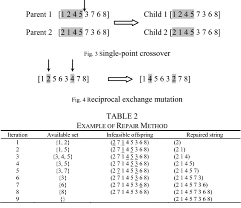
the number of chromosome pairs that will be involved in the crossover operation. For this study, a single-point crossover technique was considered. It is a simple one that combines two parent chromosomes to generate two offspring. To achieve this, the first section is directly copied into the child from the first parent; the remaining genes are obtained from the second one. The process is then repeated in reverse order to produce the second child (see Fig. 3).
2) Reciprocal exchange mutation
Mutation is a GA operation which creates new individuals by making changes in a single individual. The reciprocal exchange mutation is used. It starts by selecting two points at random and then swaps them. This is illustrated by Fig. 4 [11].
C. Repair process
An assembly line balancing problem had been developed from bin-package problem. The precedence constraint was separated them into two categories (bin-package and assembly line balancing). When genetic operator had been directly performed, it might produce infeasible offspring, resulting to the precedence constraints violation. So, a repair mechanism was required to fixes it that made the offspring became feasible. The repair procedure of K. K. Yeo et al. [6] was simple but effective. It is the same way to generate an initial feasible sequence presented in section III.A, except for Step 3, which is replaced by the following;
Step 3: among the tasks in the available set, select the task that is placed at the earliest position in the infeasible offspring, and appends it to the string.
[image:3.595.46.288.582.790.2]The Table 2 shows the step-by-step results of the repair method. An example of infeasible offspring (2 7 1 4 5 3 6 8) is shown here below.
Fig. 3 Single-point crossover
Fig. 4 Reciprocal exchange mutation
TABLE 2
EXAMPLE OF REPAIR METHOD
Iteration Available set Infeasible offspring Repaired string
1 {1, 2} (2 7 1 4 5 3 6 8) (2)
2 {1, 5} (2 7 1 4 5 3 6 8) (2 1)
3 {3, 4, 5} (2 7 1 4 5 3 6 8) (2 1 4)
4 {3, 5} (2 7 1 4 5 3 6 8) (2 1 4 5)
5 {3, 7} (2 7 1 4 5 3 6 8) (2 1 4 5 7)
6 {3} (2 7 1 4 5 3 6 8) (2 1 4 5 7 3)
7 {6} (2 7 1 4 5 3 6 8) (2 1 4 5 7 3 6)
8 {8} (2 7 1 4 5 3 6 8) (2 1 4 5 7 3 6 8)
9 {} (2 1 4 5 7 3 6 8)
D. Decoding
A sequence-oriented representation does not break precedence constraints. It is called a feasible sequence. The feasible sequence carries many possible task assignments rather than one fixed assignment. In order to determine the best assignment, the string should be properly decoded [6]. For SALBP-I, the cycle time was given. A workstation is created, and the tasks are assigned to the workstation in the order that they appear in a feasible sequence while not violating the cycle time constraint. It is repeated until all the tasks are allotted. The decoding method in this article is presented as follows.
Step 1: create empty workstation j by set j=1. Step 2: calculate Tj+TMi of the earliest gene, where Tjis the sum of
tasks time in workstation j, and TMi is execution time of task
i. Step 3: if Tj+TMi of the earliest gene is less than
predetermined cycle time, then go to step 4, otherwise go to step 6. Step 4: pack the earliest genes to workstation j, then update chromosome by removing the earliest gene, so the next gene becomes the earliest gene. Step 5: terminate, if the earliest genes is depleted. Otherwise, go to step 2. 6: set j = j+1 and go to step 1.
E. Fitness evaluation of quality-related assembly line
balancing problem
In this article, the performance measures are considered by the labor cost, the balance delay, and the quality of assembled product would be considered further. Accordingly, it is multi-objective optimization problem. One of the simplest methods for combining multiple objective functions into a scalar fitness solution was the weighted-sum approach [11]. If there are q objective functions to be maximized, the combined fitness function z is represented by:
∑
=
=
qk k
k
f
x
w
z
1
)
(
(1)If constant weights are used to calculate z, the search direction in the GA is also constant. Therefore, the random weighted approach is proposed. The wk is computed by (2)
∑
==
qj j
k
k
r
r
w
/
1 , k=1, 2,…, q (2) where rjis nonnegative random number. The q random realnumbers generated for the weights wk are used to calculate
the weighted sum z. The wk terms are varied, so the selection
probability of each string is also varied. This results in various search directions in multi-objective genetic algorithm.
Parent 1 [1 2 4 5 3 7 6 8] Child 1 [1 2 4 5 7 3 6 8]
Parent 2 [2 1 4 5 7 3 6 8] Child 2 [2 1 4 5 3 7 6 8]
[1 2 5 6 3 4 7 8]
The equation (3) shown below is the objective function (fitness function) which is taken into account the labor cost, the balance delay, and the quality of assembled product which are the multi-objectives in this study.
[1 4 5 6 3 2 7 8]
)
(
_
z
w
cC
rw
bB
rw
qQ
rMax
=
∑
+
+
(3) where, Cr is labor cost relative index, Br is balance delayrelative index, Qr is total time between quality-related tasks
relative index, wcis weight of parameter Cr, wb is weight of
parameter Br, and wc is weight of parameter Qr. By the way,
shown in (3) indicated their relative importance of the particular criteria which are predefined by (2).
1) Relative Index
The relative index is computed by (4).
)
/(C B Q
C
Cr = + + ,Br=B/(C+B+Q),Qr=Q/(C+B+Q) (4)
2) Labor Cost (C)
The equation (5) shown below is the labor cost index.
% 100 ) / ) ((
_Cost = N−Nt Nt ×
Labor (5)
where, Nt was the theoretical number of workstations which
are computed as Nt = Total assembly time/predetermine cycle
time, N is total number of workstations. So, if the computed workstations number is more than the theoretical one, the labor cost would be much more than it too.
3) Balance Delay (B)
The balance delay is the conversion value of the line efficiency. The equation (6) shown below is the computational method of the balance delay.
% 100 ) / )
(( − ×
= NCt Tt NCt
BD (6) where, Ttis total assembly time.
4) Total time between quality-related tasks
To maintain the quality level of assembled products, the time between task number x and task number y are kept because of its quality constraint. The equation (7) shown below is the computational method of total time between quality-related jobs
y x b
a
j j
y
x TN TM TM
T =
∑
− −=
− (7)
where, Tx-y is the total time between task x and y, TNj is
execution time of workstation j, and a was the workstation of
xth task, b was the workstation of yth task. TM
x and TMy are
execution time of task x, and y respectively.
F. Selection process
The Darwinian natural selection is the essential principle behind GA [11]. For this study, roulette wheel selection, proposed by Holland, is used as the main chromosome selection technique. It is an elitist approach in which the best chromosome has a highest probability to be selected for the new generation. The basic roulette wheel is a stochastic sampling with replacement. The higher evaluation function value a chromosome has, the greater potential and it will be selected as a member of the new generation. The new generation has the same population size as the previous one. With the elitist selection, the best chromosome is firstly selected for inclusion in the new generation. The selection probability pi is presented below.
∑
=−
−
=
i popsizej ji
z
z
z
z
p
(
min)
/
1(
min)
(8) where, zmin is the worst fitness value in the chromosome pool.The best chromosome is registered after the selection process. Then, update the gen value (gen=gen+1). Repeat GA procedure until gen=Maxgen.
IV. CASE COMPUTATIONAL EXPERIMENTS
The home electrical appliance manufacturer having a turn over more than 3 million US dollar per year was the case
study. The assembly line was created by line leader and experienced worker. The line efficiency was neglected, the throughput was more emphasis. Therefore, the resource utilization was low and the quality of assembled product is a big problem.
Fig. 5 shows the precedence diagram to assembly a home electrical kettle product (top product model), which is selected in this study. The 4th task (applying silicone) and the
12th (setting a thermostat) are the two tasks which are related
to a quality of assembled product. The total time between these tasks also become the interested factor because its quality is depended on silicone self-setting.
Table 3 shows the current assembly line; which was designed by production manager and line leader. From the data, the number of workstations is 17, the line efficiency is 54.55%, and the time between task 4th and 12th is 55.74 sec.
Also, the utilization of workstation is between 23.74%-100%, only 4 of them are above 70%, 10 of them are below 50%. The daily output is 996 sets.
A. Index Scalar
Further to the brainstorming with production manager and line leader, the index value was defined. Table 4 presents the value of index C of computed workstation number which is more than the theoretical one. Table 5 and 6 present the value of index B and Q respectively.
B. Analysis of Genetic parameters
When applying GA, it is known that the quality of the solution and the effectiveness of GA are likely to be influenced by the setting parameters. A computational experiment is conducted to investigate on the effects of the initial population (Popsize), generation (Maxgen), crossover probability (Pc), and mutation probability (Pm). The level of
each parameter was adopted from preliminary studies [12]-[14].
TABLE 3
CURRENT ASSEMBLY PROCESS
Workstation no. Tasks no. Utilization (%)
1 4-2 46.02
2 3 31.28
3 6-7 47.06
4 10 34.15
5 8 52.91
6 12 31.00
7 9 52.25
8 13-17 100
9 1-5 23.74
10 18-21-22 93.39
11 11-14 47.92
12 15-19-20 95.22
13 16-23-24 99.10
14 26 49.10
15 25-29 40.24
16 27-28-30 57.61
17 31-32 26.30
TABLE 4 THE LABOR COST INDEX VALUE
Labor Cost Index Value (C) Condition
5 When the Labor_Cost is 0%
4 When the Labor_Cost between 0.1-5.0%
3 When the Labor_Cost between 5.1-10.0%
2 When the Labor_Cost between 10.1-15.0%
1 When the Labor_Cost is over than 15.0%
TABLE 5
THE BALANCE DELAY INDEX VALUE
Balance Delay Index Value (B) Condition
5 When BD is between 0-4.0%
4 When BD is between 4.1-8.0%
3 When BD is between 8.1-12.0%
2 When BD is between 12.1-16.0%
3.66 1
Fig. 5 Precedence diagram of the home electrical kettle (top product model)
TABLE 6
THE TOTAL TIME BETWEEN QUALITY-RELATED TasksINDEX VALUE
Total time between quality-related jobs Index Value (Q) Condition
5 When the T4-12 is more than 96.0 sec.
4 When the T4-12 is between 72.1-96.0 sec.
3 When the T4-12 is between 48.1-72.0 sec.
2 When the T4-12 is between 24.0-48.0 sec.
1 When the T4-12 is less than 24.0 sec.
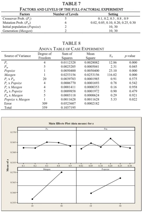
The experiment was designed as a full factorial experiment because it was more efficient and necessary to avoid misleading conclusion when interactions might be present. This technique allowed the effects of a factor to be estimated at several levels of the others, yielding conclusion was valid over the wide range [15], [16]. The experiment with four factors and three replicates is carried out. A dependent variable in this experiment is the maximum objective function (max_z). The number of levels (treatments) and the settings of each factor are shown in Table 7. There are in total of 360 runs.
ding conclusion was valid over the wide range [15], [16]. The experiment with four factors and three replicates is carried out. A dependent variable in this experiment is the maximum objective function (max_z). The number of levels (treatments) and the settings of each factor are shown in Table 7. There are in total of 360 runs.
V. RESULTS AND DISCUSSION V. RESULTS AND DISCUSSION
A two-step sequential experiment is adopted in this study. Firstly, it was aimed to initially investigate the appropriate setting of GA parameters by solving a case study of quality-related assembly line balancing problem. Its findings will be then applied in the next experiment that is aimed to design assembly line of sample factory. The development of simulation program is written by using Microsoft Visual Basic 6.0. All experiments are simulated on personal computer with CPU Intel Pentium 1.86 GHz and 512 MB of RAM.
A two-step sequential experiment is adopted in this study. Firstly, it was aimed to initially investigate the appropriate setting of GA parameters by solving a case study of quality-related assembly line balancing problem. Its findings will be then applied in the next experiment that is aimed to design assembly line of sample factory. The development of simulation program is written by using Microsoft Visual Basic 6.0. All experiments are simulated on personal computer with CPU Intel Pentium 1.86 GHz and 512 MB of RAM.
A. The results of genetic parameters analysis
A. The results of genetic parameters analysis
Analysis of Variance (ANOVA) is used to investigate the effects of the main factors and their interactions. Table 8 shows the results of this analysis (the case study is case experiment). For a given confidence levelα, all factors or interactions with a value of p≤ α are statistically significant, whilst other factors may be disregarded.
Analysis of Variance (ANOVA) is used to investigate the effects of the main factors and their interactions. Table 8 shows the results of this analysis (the case study is case experiment). For a given confidence levelα, all factors or interactions with a value of p≤ α are statistically significant, whilst other factors may be disregarded.
All of main factors have values of p≤ 0.05 and are therefore statistically significant, within the ranges considered. The first main factor, which is the probability of crossover, has effect on objective function value. Probability of mutation is also significant but less important. The last two main factors, population size and the number of generation, are also significant. The results show the objective value for population of 30 is better than that with 10 (see Fig. 6).
Likewise, 30 generations produces better results than 10. Moreover, these two factors also have interaction.
An interaction was the failure of one factor that produces the same effect on the response at different levels of another factor [16]. Table 8 and Fig. 6 show the interaction between the population size and the number of generation.
An interaction was the failure of one factor that produces the same effect on the response at different levels of another factor [16]. Table 8 and Fig. 6 show the interaction between the population size and the number of generation.
It can be explained that increasing the number of generations and population, both increasing will also increase the number of search that enables to improve solution quality. However, it was found that increasing the number of generations and population has significant effect to computational time.
[image:5.595.303.549.395.761.2]It can be explained that increasing the number of generations and population, both increasing will also increase the number of search that enables to improve solution quality. However, it was found that increasing the number of generations and population has significant effect to computational time.
TABLE 7 TABLE 7
FACTORS AND LEVELS OF THE FULL-FACTORIAL EXPERIMENT
FACTORS AND LEVELS OF THE FULL-FACTORIAL EXPERIMENT
Factors
Factors Number of Levels Number of Levels Setting Setting
Crossover Prob. (Pc) 5 0.1, 0.2, 0.3 , 0.8 , 0.9
Mutation Prob. (Pm) 6 0.02, 0.05, 0.10, 0.20, 0.25, 0.30
Initial population (Popsize) 2 10, 30
Generation (Maxgen) 2 10, 30
TABLE 8
ANOVA TABLE OF CASE EXPERIMENT
Source of Variance Degree of Freedom Squares Sum of Square Mean F0 p-value
Pc 4 0.0112328 0.0028082 12.86 0.000
Pm 5 0.0025205 0.0005041 2.31 0.045
Popsize 1 0.0050400 0.0050400 23.10 0.000
Maxgen 1 0.0253156 0.0253156 116.02 0.000
Pcx Pm 20 0.0039703 0.0001985 0.91 0.575
Pc x Popsize 4 0.0006770 0.0001693 0.78 0.542
Pc x Maxgen 4 0.0001411 0.0000353 0.16 0.958
Pm x Popsize 5 0.0009858 0.0001972 0.90 0.479
Pm x Maxgen 5 0.0003118 0.0000624 0.29 0.921
Popsize x Maxgen 1 0.0011628 0.0011628 5.33 0.022
Error 309 0.0523607 0.0002182
Total 359 0.1037195
Me a n o f z 0.9 0.8 0.3 0.2 0.1 0.370 0.365 0.360 0.355 0.30 0.25 0.20 0.10 0.05 0.02 30 10 0.370 0.365 0.360 0.355 30 10 Pc Pm Maxgen Popsize
Main Effe cts Plot (data me ans) for z
Fig. 6 The main effect plots of GA parameters
2 3 6 4 5 7 8 9
10 12
13
17
18
21 22 23
25 29
24 26
27 28
30 31 32
5.36 9.04 7.94 3.20 15.29 8.50 5.10 9.87 15.10 8.96 10.22 18.68 8.47
8.95 9.82 10.23
8.78 2.85 5.71
5.81 14.19
11 16
5.47
5.37 3.85 3.75
i
TMi where,
i is task 1,2,…,M
TMi is execution time of task i
Tt is total assembly time = 268.24 sec. 14
8.50 12.70
5.35 9.70
15 20
19
B. The results of case simulation
By decoding the chromosome of case simulation being executed by GA of which the parameters are as follows: Pc=
0.3, Pm= 0.2, Popsize= 30, Maxgen= 30, the execution time
of 139,250 ms. is satisfying. The GA results are shown in Table 9, and Table 10 shows the results comparison between GA approach and current performance.
The number of workstations of 12 is obtained, the line efficiency is 89.47%, and the time between 4th and 12th tasks
is 102.88 sec. In addition, the mentioned time above is an appropriate time because the self-setting of the silicone is perfectly complete. Also, the utilization of workstations is between 73.76%-100%, and the daily output is 1,152 sets.
By comparing the computational results obtained under random-weighted-sum combination with current production status, number of workstation is significantly decreased from 17 to 12 (see Table 10). By considering of the quality aspect generated from proposed GA model, it is shown that the quality of assembled product is better. Finally, cycle time of case study is less than the current one.
Factory Management, then, decides to change the workstations according to GA’s results. It is also resulted to decrease the manpower from 17 to 12 and to increase daily output from 996 sets to 1,152 sets.
VI. CONCLUSIONS
The combination of GA model considering quality-related product together with full-factorial experimental design of genetic parameters is shown to be an effective approach to minimize production cost while keeping good product quality of sample assembly line. Management factory was satisfied on the overall result after its improvement. Finally, engineering management and other IE techniques would be further considered and investigated to achieve more performance.
ACKNOWLEDGMENT
The authors would like to express our gratitude to employees of sample factory for their kind collaboration, and Dr. Pupong Pongcharoen, assistant professor, Naresuan University, Thailand, for his useful suggestion.
TABLE 9
COMPUTATIONAL RESULT OF GAAPPROACH
Workstation no. Tasks no. Utilization (%)
1 3-1-5-11 97.60
2 2-4-14-7 95.00
3 6-16 84.80
4 9-10 99.88
5 8-19 100
6 12-15 88.92
7 20-13-18 92.96
8 17 74.72
9 21-22 75.08
10 23-24-25 98.88
11 26-29-27 91.40
12 28-30-31-32 73.76
TABLE 10
RESULTS COMPARISON BETWEEN GAAPPROACHAND CURRENT PERFORMANCE
Current
performance GA results
Objective Function - 0.38
Number of Workstations 17 12
Line efficiency (%) 54.55 89.47
Total time between quality-related tasks (sec.) 55.74 102.88
Cycle time (max. executed time workstation) (sec./set) 28.90 24.99
Daily output (sets/day) 996 1,152
REFERENCES
[1] Jay Heizer, Barry Render, Operation Management, New Jersey: Pearson Prentice Hall, 2006, pp. 355-359.
[2] Ronald G. Askin, Jeffrey B. Goldberg, Design and Analysis of Lean Production Systems, New York: John Wiley & Sons, 2001, pp. 395-399.
[3] J. Rubinovitz, G. Levitin, “Genetic algorithm for assembly line balancing,” International Journal of Production Economics, vol.41, Issue 1-3, pp. 343-354, Oct 1995.
[4] R. Brahim, D Alexandre, D. Alain, and B. Antoneta, “State of Art of Optimization methods for Assembly Line design,” Annual Reviews in Control, vol. 26, pp. 163-174, 2002.
[5] P. Pongchareon, C. Hicks, P.M. Braiden, and D.J. Stewardson, “Determining optimum Genetic Algorithm parameters for scheduling the manufacturing and assembly of complex products,” International Journal of Productions Economics, vol. 78, pp. 311-322, 2002. [6] K. K. Yeo, J. K. Yong, and K. Yeongho, “Genetic Algorithms for
Assembly Line Balancing with Various Objectives,” Computer& Industrial Engineering, vol. 30, Issue 3, pp. 397-409, 1996.
[7] S.G. Ponnambalam, P. Aravindan, and G. Mogileeswar Naidu, “A Multi-Objective Genetic Algorithm for Solving Assembly Line Balancing Problem,” The International Journal of Advanced Manufacturing Technology, vol. 16, pp. 341-352, 2000.
[8] S. Armin, B. Christian, “State-of-the-art exact and heuristic solution procedures form simple assembly line balancing,” European Journal of Operation Research, vol. 168, pp. 666-693, 2006.
[9] R-S. Chen, K-Y. Lu, and S-C. Yu, “A hybrid genetic algorithm approach on multi-objective of assembly planning problem,”
Engineering Applications of Artificial Intelligence, vol. 15, pp.447-457, 2002.
[10] Y. Y. Leu, L. A. Matheson, and L. P. Rees, “Assembly line balancing using genetic algorithms with heuristic-generated initial populations and multiple evaluation criteria,” Decision Sciences, vol. 25, Issue 4, pp. 581-606. 1994.
[11] M. Gen, and R. Chen, Genetic Algorithms & Engineering Optimization. New York: John Wiley & Sons, 2000, pp. 124-131. [12] E. J. Anderson, M. C. Ferris, “Genetic Algorithms for Combinatorial
Optimization: The Assembly Line Balancing Problem,” Journal of Computing, vol. 6, No. 2, pp. 161-173. 1994.
[13] K. Asaarungsaengkul, and S. Nanthavanij, “A Genetic Algorithm Approach to selection of Engineering Controls for Optimal Noise Reduction,” ScienceAsia, vol.33, pp. 89-101, 2007.
[14] P. Pongchareon, W. Chainate, and P. Thapatsuwan, “Exploration of Genetic Parameters and Operators through Traveling Salesman Problem,” ScienceAsia, vol. 33, pp. 215-222, 2007.
[15] P. Pongchareon, C. Hicks, and P.M. Braiden, “The development of genetic algorithms for the finite capacity scheduling of complex products, with multiple levels of product structure,” European Journal of Operational Research, vol. 152, pp. 215-225, 2004.