Proceedings of the 2019 Conference on Empirical Methods in Natural Language Processing and the 9th International Joint Conference on Natural Language Processing, pages 1093–1104,
1093
A Bayesian Approach for Sequence Tagging with Crowds
Edwin Simpson and Iryna Gurevych
Ubiquitous Knowledge Processing Lab Department of Computer Science Technische Universit¨at Darmstadt
https://www.ukp.tu-darmstadt.de
{simpson,gurevych}@ukp.informatik.tu-darmstadt.de
Abstract
Current methods for sequence tagging, a core task in NLP, are data hungry, which motivates the use of crowdsourcing as a cheap way to obtain labelled data. However, annotators are often unreliable and current aggregation meth-ods cannot capture common types of span an-notation errors. To address this, we propose a Bayesian method for aggregating sequence tags that reduces errors by modelling sequen-tial dependencies between the annotations as well as the ground-truth labels. By taking a Bayesian approach, we account for unctainty in the model due to both annotator er-rors and the lack of data for modelling anno-tators who complete few tasks. We evaluate our model on crowdsourced data for named entity recognition, information extraction and argument mining, showing that our sequential model outperforms the previous state of the art. We also find that our approach can re-duce crowdsourcing costs through more effec-tive aceffec-tive learning, as it better captures un-certainty in the sequence labels when there are few annotations.
1 Introduction
Current methods forsequence tagging, a core task in NLP, use deep neural networks that require tens of thousands of labelled documents for training (Ma and Hovy,2016;Lample et al.,2016). This presents a challenge when facing new domains or tasks, where obtaining labels is often time-consuming or costly. Labelled data can be ob-tained cheaply by crowdsourcing, in which large numbers of untrained workers annotate documents instead of more expensive experts. For sequence tagging, this results in multiple sequences of unre-liable labels for each document.
Probabilistic methods for aggregating crowd-sourced data have been shown to be more accu-rate than simple heuristics such as majority
vot-ing (Raykar et al., 2010; Sheshadri and Lease,
2013;Rodrigues et al.,2013;Hovy et al.,2013). However, existing methods for aggregating se-quence labels cannot model dependencies between the annotators’ labels (Rodrigues et al., 2014;
Nguyen et al.,2017) and hence do not account for their effect on annotator noise and bias. In this paper, we remedy this by proposing a sequential annotator model and applying it to tasks that fol-low abeginning, inside, outside(BIO) scheme, in which the first token in a span of type ‘x’ is la-belled ‘B-x’, subsequent tokens are lala-belled ‘I-x’, and tokens outside spans are labelled ‘O’.
When learning from noisy or small datasets, commonly-used methods based on maximum like-lihood estimation may produce over-confident pre-dictions (Xiong et al., 2011; Srivastava et al.,
2014). In contrast, Bayesian inference accounts for model uncertainty when making predictions. Unlike alternative methods that optimize the val-ues for model parameters, Bayesian inference in-tegrates over all possible values of a parame-ter, weighted by a prior distribution that captures background knowledge. The resulting posterior probabilities improve downstream decision mak-ing as they include the probability of errors due to a lack of knowledge. For example, during ac-tive learning, posterior probabilities assist with se-lecting the most informative data points (Settles,
2010).
In this paper, we develop Bayesian sequence combination (BSC), building on prior work that has demonstrated the advantages of Bayesian inference for aggregating unreliable classifica-tions (Kim and Ghahramani,2012;Simpson et al.,
of annotator noise and bias, which goes beyond previous work by modelling sequential dependen-cies between annotators’ labels. Further contribu-tions include a theoretical comparison of the prob-abilistic models of annotator noise and bias, and an empirical evaluation on three sequence labelling tasks, in whichBSC withseqconsistently outper-forms the previous state of the art. We make all of our code and data freely available1.
2 Related Work
Sheshadri and Lease (2013) benchmarked several aggregation models for non-sequential classifica-tions, obtaining the most consistent performance from that of Raykar et al. (2010), who model the reliability of individual annotators using proba-bilistic confusion matrices, as proposed by Dawid and Skene (1979). Simpson et al. (2013) showed that a Bayesian variant of Dawid and Skene’s model can outperform maximum likelihood ap-proaches and simple heuristics when combining crowds of image annotators. This Bayesian vari-ant, independent Bayesian classifier combination (IBCC) (Kim and Ghahramani, 2012), was orig-inally used to combine ensembles of automated classifiers rather than human annotators. While traditional ensemble methods such as boosting fo-cus on how to generate new classifiers (Dietterich,
2000), IBCC is concerned with modelling the re-liability of each classifier in a given set of clas-sifiers. To reduce the number of parameters in multi-class problems, Hovy et al. (2013) proposed MACE, and showed that it performed better un-der a Bayesian treatment on NLP tasks. Paun et al. (2018) further illustrated the advantages of Bayesian models of annotator ability on NLP clas-sification tasks with different levels of annotation sparsity and noise.
We expand this previous work by detailing the relationships between several annotator models and extending them to sequential classification. Here we focus on the core annotator representa-tion, rather than extensions for clustering annota-tors (Venanzi et al., 2014; Moreno et al., 2015), modeling their dynamics (Simpson et al., 2013), adapting to task difficulty (Whitehill et al.,2009;
Bachrach et al., 2012), or time spent by annota-tors (Venanzi et al.,2016).
Methods for aggregating sequence labels
in-1http://github.com/ukplab/ arxiv2018-bayesian-ensembles
clude CRF-MA (Rodrigues et al., 2014), a CRF-based model that assumes only one annotator is correct for any given label. Recently, Nguyen et al. (2017) proposed a hidden Markov model (HMM) approach that outperformed CRF-MA, called HMM-crowd. Both CRF-MA and HMM-crowd use simpler annotator models than Dawid and Skene (1979) that do not capture the effect of sequential dependencies on annotator reliabil-ity. Neither CRF-MA nor HMM-crowd use a fully Bayesian approach, which has been shown to be more effective for handling uncertainty due to noise in crowdsourced data for non-sequential classification (Kim and Ghahramani,2012; Simp-son et al., 2013; Venanzi et al., 2014; Moreno et al.,2015). In this paper, we develop a sequen-tial annotator model and an approximate Bayesian method for aggregating sequence labels.
3 Modeling Sequential Annotators
When combining multiple annotators with varying skill levels, we can improve performance by mod-elling their individual noise and bias using a prob-abilistic model. Here, we describe several models that do not consider dependencies between anno-tations in a sequence, before definingseq, a new extension that captures sequential dependencies. Probabilistic annotator models each define a dif-ferent function, A, for the likelihood that the an-notator chooses labelcτgiven the true labeltτ, for theτth token in a sequence.
Accuracy model (acc): the basis of several pre-vious methods (Donmez et al., 2010; Rodrigues et al.,2013),accuses a single parameter for each annotator’s accuracy,π:
A=p(cτ=i|tτ=j, π) = (
π wherei=j 1−π
J−1 otherwise )
,
(1)
whereJis the number of classes. This may be un-suitable when one class label dominates the data, since a spammer who always selects the most common label will nonetheless have a highπ.
the true label,tτ.
A=p(cτ =i|tτ =j, π,ξ)
=
(
π+ (1−π)ξj wherei=j (1−π)ξj otherwise
)
. (2)
This addresses the case where spammers choose the dominant label but does not explicitly model different error rates in each class. For example, if an annotator is better at detecting type ‘x’ spans than type ‘y’, or if they frequently miss the first token in a span, thereby labelling the start of a span as ‘O’ when the true label is ‘B-x’, this would not be explicitly modelled byspam.
Confusion vector (CV): this approach learns a separate accuracy for each class label (Nguyen et al.,2017) using parameter vector,π, of sizeJ:
A=p(cτ=i|tτ=j,π) = (
πj wherei=j 1−πj
J−1 otherwise )
.
(3)
This model does not capture spamming patterns where one of the incorrect labels has a much higher likelihood than the others.
Confusion matrix (CM) (Dawid and Skene,
1979): this model can be seen as an expansion of the confusion vector so thatπ becomes aJ ×J matrix with values given by:
A=p(cτ=i|tτ=j,π) =πj,i. (4)
This requires a larger number of parameters, J2, compared to theJ + 1parameters of MACE orJ parameters of the confusion vector. Like spam, CM can model spammers who frequently chose one label regardless of the ground truth, but also models different error rates and biases for each class. However, CM ignores dependencies be-tween annotations in a sequence, such as the fact that an ‘I’ cannot immediately follow an ‘O’.
Sequential Confusion Matrix (seq): we intro-duce a new extension to the confusion matrix to model the dependency of each label in a sequence on its predecessor, giving the following likelihood:
A=p(cτ=i|cτ−1=ι, tτ=j,π) =πj,ι,i, (5)
whereπ is now three-dimensional with size J × J ×J. In the case of disallowed transitions, e.g. fromcτ−1 =‘O’ tocτ =‘I’, the valueπj,cτ−1,cτ ≈ 0, ∀j is fixed a priori. The sequential model can capture phenomena such as a tendency toward
overly long sequences, by learning that I is more likely to follow another I, so thatπO,I,I > πO,I,O. A tendency to split spans by inserting ‘B’ in place of ‘I’ can be modelled by increasing the value of πI,I,Bwithout affectingπI,B,B andπI,O,B.
The annotator models presented in this section include the most widespread models for NLP an-notation tasks, and can be seen as extensions of one another. The choice of annotator model for a particular annotator depends on the developer’s understanding of the annotation task: if the anno-tations have sequential dependencies, this suggests the seq model; for non-sequential classifications CM may be effective with small (≤ 5) numbers of classes;spammay be more suitable if there are many classes, as the number of parameters to learn is low. However, there is also a trade-off between the expressiveness of the model and the number of parameters that must be learned. Simpler mod-els with fewer parameters may be effective if there are only small numbers of annotations from each annotator. The next section shows how these an-notator models can be used as components of a complete model for aggregating sequential anno-tations.
4 A Generative Model for Bayesian Sequence Combination
To construct a generative model forBayesian se-quence combination (BSC), we first define a hid-den Markov model (HMM) with states tn,τ and observationsxn,τ using categorical distributions:
tn,τ ∼Cat(Ttn,τ−1), (6)
xn,τ ∼Cat(ρtn,τ), (7)
where Tj is a row of a transition matrix T, and ρj is a vector of observation likelihoods for state j. For text tagging, n indicates a document and τ a token index, while each state tn,τ is a true sequence label and xn,τ is a token. To provide a Bayesian treatment, we assume thatTj andρj have Dirichlet distribution priors as follows:
Tj ∼Dir(γj), ρj ∼Dir(κj), (8)
whereγjandκj are hyperparameters.
our experiments in Section6, we compare differ-ent choices of annotator model as compondiffer-ents of BSC. All the parameters of these annotator models are probabilities, so to provide a Bayesian treat-ment, we assume that they have Dirichlet priors. For annotatork’s annotator model, we refer to the hyperparameters of its Dirichlet prior asα(k). The annotator model defines a categorical likelihood over each annotation,c(k)n,τ:
c(k)n,τ ∼Cat([A(k)(tn,τ,1,c(k)n,τ−1), ...,
A(k)(tn,τ, J,c(k)n,τ−1)]). (9)
The annotators are assumed to be conditionally independent of one another given the true labels, t, which means that their errors are assumed to be uncorrelated. This is a strong assumption when considering that the annotators have to make their decisions based on the same input data. However, in practice, dependencies do not usually cause the most probable label to change (Zhang,2004), hence the performance of classifier combination methods is only slightly degraded, while avoid-ing the complexity of modellavoid-ing dependencies be-tween annotators (Kim and Ghahramani,2012).
Joint distribution: the complete model can be represented by the joint distribution, given by:
p(t,A,T,ρ,c,x|α(1), ...,α(K),γ,κ) (10)
= K Y
k=1 (
p(A(k)|α(k)) N Y
n=1
p(c(k)n |A(k),t)
)
N Y
n=1 Ln Y
τ=1
p(tn,τ|Ttn,τ−1)p(xn,τ|tn,τ,ρtn,τ)
J Y
j=1
p(Tj|γj)p(ρj|κj) (11)
wherecis the set of annotations for all documents from all annotators,tis the set of all sequence la-bels for all documents,N is the number of docu-ments,Lnis the length of thenth document,J is the number of classes,xis the set of all word se-quences for all documents andρ,γandκare the sets of parameters for all label classes.
5 Inference using Variational Bayes
Given a set of annotations,c, we obtain a posterior distribution over sequence labels, t, using varia-tional Bayes (VB) (Attias, 2000). Unlike maxi-mum likelihood methods such as standard
expec-tation maximization (EM), VB considers prior dis-tributions and accounts for parameter uncertainty due to noisy or sparse data. In comparison to other Bayesian approaches such as Markov chain Monte Carlo (MCMC), VB is often faster, read-ily allows incremental learning, and provides eas-ier ways to determine convergence (Bishop,2006). It has been successfully applied to a wide range of methods, including being used as the standard learning procedure for LDA (Blei et al.,2003), and to combining non-sequential crowdsourced classi-fications (Simpson et al.,2013).
The trade-off is that we must approximate the posterior distribution with an approximation that factorises between subsets of latent variables:
p(t,A,T,ρ|c,x,α,γ,κ)
≈ K Y
k=1
q(A(k)) J Y
j=1
q(Tj)q(ρj) N Y
n=1 q(tn).
(12)
VB performs approximate inference by updating each variational factor, q(z), in turn, optimising the approximate posterior distribution until it con-verges. Details of the theory are beyond the scope of this paper, but are explained by Bishop(2006). The VB algorithm is described in Algorithm 1, making use of update equations for the variational factors given below.
Input: Annotationsc, tokensx
1 Compute initial values ofElnA(k),∀k, Elnρj,∀j,ElnTj,∀jfrom their prior distributions.
whilenot converged(rn,τ,j,∀n,∀τ,∀j)do
2 Updaterj,n,τ,stj,n,τ−1,tι,n,τ,∀j,∀τ,∀n,∀ι,
using forward-backward algorithm given x,c,ElnTj,∀j,Elnρj,∀j,
ElnA(k),∀k.
3 UpdateElnA(k),∀k, givenc,rj,n,τ. 4 UpdateElnTj,ι,∀j,∀ι, given
stj,n,τ−1,tι,n,τ.
5 UpdateElnρj,∀jgivenx,rj,n,τ. end
Output: Label posteriors,rn,τ,j,∀n,∀τ,∀j, most probable sequence of labels, ˆtn,∀nusing Viterbi algorithm
Algorithm 1:The VB algorithm for BSC.
of each label transition, sn,τ,j,ι = E[p(tn,τ−1 = j, tn,τ = ι|c)], using the forward-backward algo-rithm (Ghahramani, 2001). In the forward pass, we compute:
lnrn,τ,j− = ln J X
ι=1 n
r−n,τ−1,ιeElnTι,j o
+lln,τ(j),
lln,τ(j) = K X
k=1
ElnA(k)
j, c(k)n,τ, c(k)n,τ−1
Elnρj,xn,τ,
(13)
and in the backward pass we compute:
lnλn,τ,j = ln J X
ι=1 exp
lnλi,τ+1,ι
+ElnTj,ι+lln,τ+1(ι) . (14)
Then we can calculate the posteriors as follows:
rn,τ,j ∝r−n,τ,jλn,τ,j, (15)
sn,τ,j,ι∝r−n,τ−1,jλn,τ,ιexp{ElnTj,ι+lln,τ(ι)}. (16)
The expectations of lnT andlnρcan be com-puted using standard equations for a Dirichlet dis-tribution:
ElnTj,ι= Ψ(Nj,ι+γj,ι)−Ψ
J X
i=1
(Nj,i+γj,i) !
,
(17)
Elnρj = Ψ(oj,w+κj,w)−Ψ
J X
v=1
(oj,v+κj,v) !
,
(18)
where Ψ is the digamma function, Nj,ι =
PN
n=1 PLn
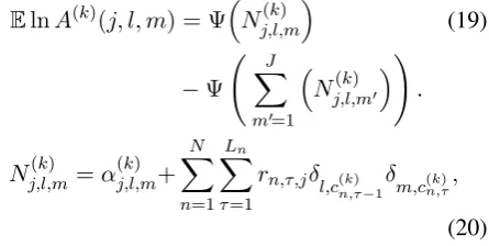
τ=1sn,τ,j,ι is the expected number of times that label ιfollows label j, and oj,w is the expected number of times that wordwoccurs with sequence labelj. Similarly, for theseqannotator model, the expectation terms are:
ElnA(k)(j, l, m) = Ψ
Nj,l,m(k)
(19)
−Ψ J X
m0=1
Nj,l,m(k) 0
!
.
Nj,l,m(k) =α(k)j,l,m+ N X
n=1 Ln X
τ=1
rn,τ,jδl,c(k)
n,τ−1
δ m,c(n,τk),
(20)
whereδis the Kronecker delta. For other annota-tor models, this equation is simplified as the values of the previous labelsc(k)n,τ−1 are ignored.
[image:5.595.68.291.608.720.2]data #sentences or docs #annotators #gold span -set total dev test total /doc spans length NER 6,056 2,800 3,256 47 4.9 21,612 1.51 PICO 9,480 191 191 312 6.0 700 7.74 ARG 8,000 60 100 105 5 73 17.52
Table 1: Dataset statistics. Span lengths are means.
5.1 Most Likely Sequence Labels
The approximate posterior probabilities of the true labels,rj,n,τ, provide confidence estimates for the labels. However, it is often useful to compute the most probable sequence of labels, ˆtn, using the Viterbi algorithm (Viterbi,1967). The most prob-able sequence is particularly useful because, un-likerj,n,τ, the sequence will be consistent with any transition constraints imposed by the priors on the transition matrix T, such as preventing ‘O’→‘I’ transitions by assigning them zero probability.
6 Experiments
Datasets. We compare BSC to alternative meth-ods on three NLP datasets containing both crowdsourced and gold sequential annotations. NER, the CoNLL 2003 named-entity recognition dataset (Tjong Kim Sang and De Meulder,2003), which contains gold labels for four named en-tity categories (PER, LOC, ORG, MISC), with crowdsourced labels provided by (Rodrigues et al.,
2014). PICO (Nguyen et al., 2017), consists of medical paper abstracts that have been annotated by a crowd to indicate text spans that identify the population enrolled in a clinical trial.ARG( Traut-mann et al.,2019) contains a mixture of argumen-tative and non-argumenargumen-tative sentences, in which the task is to mark the spans that contain pro or con arguments for a given topic. Dataset statistics are shown in Table 1. The datasets differ in typical span length, with argument components in ARG the longest, while named entities in NER spans are often only one token long.
The gold-labelled documents are split into val-idation and test sets. For NER, we use the split given by Nguyen et al. (2017), while for PICO and ARG, we make random splits since the splits from previous work were not available2.
Evaluation metrics. For NER and ARG we use the CoNLL 2003 F1-score, which considers only
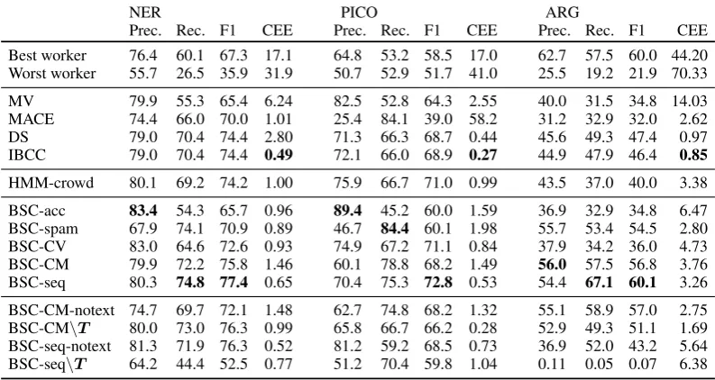
NER PICO ARG
Prec. Rec. F1 CEE Prec. Rec. F1 CEE Prec. Rec. F1 CEE Best worker 76.4 60.1 67.3 17.1 64.8 53.2 58.5 17.0 62.7 57.5 60.0 44.20 Worst worker 55.7 26.5 35.9 31.9 50.7 52.9 51.7 41.0 25.5 19.2 21.9 70.33
MV 79.9 55.3 65.4 6.24 82.5 52.8 64.3 2.55 40.0 31.5 34.8 14.03 MACE 74.4 66.0 70.0 1.01 25.4 84.1 39.0 58.2 31.2 32.9 32.0 2.62 DS 79.0 70.4 74.4 2.80 71.3 66.3 68.7 0.44 45.6 49.3 47.4 0.97 IBCC 79.0 70.4 74.4 0.49 72.1 66.0 68.9 0.27 44.9 47.9 46.4 0.85
HMM-crowd 80.1 69.2 74.2 1.00 75.9 66.7 71.0 0.99 43.5 37.0 40.0 3.38
BSC-acc 83.4 54.3 65.7 0.96 89.4 45.2 60.0 1.59 36.9 32.9 34.8 6.47 BSC-spam 67.9 74.1 70.9 0.89 46.7 84.4 60.1 1.98 55.7 53.4 54.5 2.80 BSC-CV 83.0 64.6 72.6 0.93 74.9 67.2 71.1 0.84 37.9 34.2 36.0 4.73 BSC-CM 79.9 72.2 75.8 1.46 60.1 78.8 68.2 1.49 56.0 57.5 56.8 3.76 BSC-seq 80.3 74.8 77.4 0.65 70.4 75.3 72.8 0.53 54.4 67.1 60.1 3.26
[image:6.595.100.497.64.275.2]BSC-CM-notext 74.7 69.7 72.1 1.48 62.7 74.8 68.2 1.32 55.1 58.9 57.0 2.75 BSC-CM\T 80.0 73.0 76.3 0.99 65.8 66.7 66.2 0.28 52.9 49.3 51.1 1.69 BSC-seq-notext 81.3 71.9 76.3 0.52 81.2 59.2 68.5 0.73 36.9 52.0 43.2 5.64 BSC-seq\T 64.2 44.4 52.5 0.77 51.2 70.4 59.8 1.04 0.11 0.05 0.07 6.38
Table 2: Aggregating crowdsourced labels: estimating true labels for documents labelled by the crowd.
exact span matches to be correct. Incomplete named entities are typically not useful, and for ARG, it is desirable to identify complete argumen-tative units that make sense on their own. For med-ical trial populations, partial matches still contain useful information, so for PICO we use a relaxed F1-score, as in Nguyen et al.(2017), which counts the matching fractions of spans when computing precision and recall.
We also compute the cross entropy error (CEE, also known as log-loss). While this is a token-level rather than span-level metric, it evaluates the qual-ity of the probabilqual-ity estimates produced by aggre-gation methods, which are useful for tasks such as active learning, as it penalises over-confident mis-takes more heavily.
Evaluated Methods. We evaluate BSC in com-bination with all of the annotator models described in Section 4. As well-established non-sequential baselines, we include token-level majority voting (MV),MACE (Hovy et al., 2013) which uses the spamannotator model, Dawid-Skene (DS) (Dawid and Skene, 1979), which uses the CM anno-tator model, and independent Bayesian classi-fier combination (IBCC) (Kim and Ghahramani,
2012), which is a Bayesian treatment of Dawid-Skene. We also compare against the state-of-the-art sequentialHMM-crowdmethod (Nguyen et al.,
2017), which uses a combination of maximuma posteriori(or smoothed maximum likelihood) es-timates for theCVannotator model and variational inference for an integrated hidden Markov model
(HMM). HMM-Crowd and DS use non-Bayesian inference steps and can be compared with their Bayesian variants, BSC-CV and IBCC, respec-tively.
Besides the annotator models, BSC also makes use of text features and a transition matrix,T, over true labels. We test the effect of these components by running BSC-CM and BSC-seq with no text features (notext), and without the transition ma-trix, which is replaced by simple independent class probabilities (labelled\T).
We tune the hyperparameters using grid search on the development sets. To limit the number of hyperparameters to tune, we optimize only three values for BSC: hyperparameters of the transition matrix, γj, are set to the same value, γ0, except for disallowed transitions, (O I and transitions be-tween types, e.g. I-PER I-ORG), which are set to 1e− 6; for the annotator models, all values are set to α0, except for disallowed transitions, which are set to1e−6, then0 is added to hyper-parameters corresponding to correct annotations (e.g. diagonal entries in a confusion matrix). This encodes the prior assumption that annotators are more likely to have an accuracy greater than ran-dom, which avoids the non-identifiability problem in which the class labels are switched around.
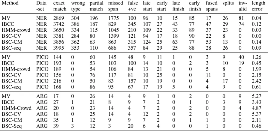
(sig-Method Data exact wrong partial missed false late early late early fused splits inv- length -set match type match span +ve start start finish finish spans alid error
MV NER 2869 304 196 1775 100 96 10 15 85 17 26 81 0.04 IBCC NER 3742 386 187 829 345 107 27 43 77 47 29 74 0.12 HMM-crowd NER 3650 334 115 1045 210 109 22 33 89 37 23 0 0.03 BSC-CV NER 3381 284 80 1399 121 94 17 18 90 22 8 0 0.00 BSC-CM NER 3856 362 63 863 315 124 25 63 77 53 13 0 0.14 BSC-seq NER 3995 353 110 686 357 84 29 25 88 28 26 0 0.09
MV PICO 144 0 60 145 48 9 11 1 0 3 9 40 1.26 IBCC PICO 193 0 53 103 100 14 10 0 2 3 10 19 0.45 HMM-crowd PICO 189 0 54 106 84 13 21 0 0 5 8 0 1.99 BSC-CV PICO 156 0 76 117 81 10 25 0 0 11 0 0 2.15 BSC-CM PICO 216 0 50 83 157 10 19 0 0 4 17 0 2.42 BSC-seq PICO 168 0 86 95 67 17 19 5 0 4 9 0 0.61
MV ARG 17 0 26 14 4 9 1 0 2 0 0 9 5.27
[image:7.595.76.523.66.285.2]IBCC ARG 27 1 21 8 9 7 2 0 1 0 3 9 3.43 HMM-Crowd ARG 20 0 23 14 4 7 2 0 2 0 0 4 4.87 BSC-CV ARG 18 0 25 14 4 12 2 0 2 0 0 0 5.37 BSC-CM ARG 35 1 12 9 9 7 2 0 1 1 0 0 2.11 BSC-Seq ARG 39 3 12 3 20 6 4 0 0 1 0 0 0.46
Table 3: Counts of different types of span errors.
nificant on all datasets with p .01 using a two-tailed Wilcoxon signed-rank test). Without the text model (BSC-seq-notext) or the transition matrix (BSC-seq\T), BSC-seq performance de-creases heavily, while CM-notext and BSC-CM\T in some cases outperform BSC-CM. This suggests that seq, with its greater number of pa-rameters to learn, is most effective in combination with the transition matrix and simple text model. On the ARG dataset, the scores are close to zero for BSC-seq\T. Further investigation shows that this is because BSC-seq\T identifies many spans with one or two incorrect labels. Since we use ex-act span matches to compute true and false pos-itives, these small errors reduce the scores sub-stantially. In particular, we find a large number of missing B tags at the start of spans and misplaced O tags that split spans in the middle.
The performance of all methods across the three datasets varies greatly. With NER, the spans are short and the task is less subjective than PICO or ARG, hence its higher F1 scores. PICO uses a re-laxed F1 score, meaning its scores are only slightly lower despite being a more ambiguous task. The constitution of an argument is also ambiguous, so ARG scores are lower, particularly as we use strict span-matching to compute the F1 scores. Raising the scores may be possible in future by using ex-pert labels as training data, i.e. as known values of t, which would help to put more weight on anno-tators with similar labelling patterns to the experts. We categorise the errors made by key methods
and list the counts for each category in Table 3. All machine learning methods tested here reduce the number of spans that were completely missed by majority voting. Note that BSC completely re-moves all “invalid” spans (O I transitions) due to the sequential model with prior hyperparameters set to zero for those transitions. For PICO and ARG, which contain longer spans, BSC-seq has lower “length error” than other methods, which is the mean difference in number of tokens between the predicted and gold spans. It also reduces the number of missing spans, although in NER and ARG that comes at the cost of producing more false positives (predicting spans where there are none). Overall, BSC-seq appears to be the best choice for identifying exact span matches and re-ducing missed spans.
varia-Previous label = I:
I O B annotator label I
O B
true label
Cluster 0
I O B I
O B
Cluster 1
I O B I
O B
Cluster 2
I O B I
O B
Cluster 3
I O B I
O B
Cluster 4
Previous label = O:
I O B annotator label I
O B
true label
Cluster 0
I O B I
O B
Cluster 1
I O B I
O B
Cluster 2
I O B I
O B
Cluster 3
I O B I
O B
Cluster 4
Previous label = B:
I O B annotator label I
O B
true label
Cluster 0
I O B I
O B
Cluster 1
I O B I
O B
Cluster 2
I O B I
O B
Cluster 3
I O B I
O B
Cluster 4
0.5 0.0 0.5 1.0 1.5
0.50 0.25 0.00 0.25 0.50 0.75 1.00 1.25 1.50
0.0 0.2 0.4 0.6 0.8 1.0
[image:8.595.70.529.64.364.2]0.0 0.2 0.4 0.6 0.8 1.0
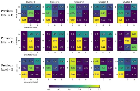
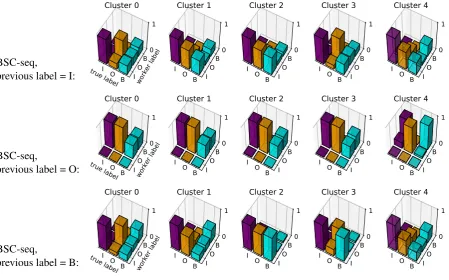
Figure 1: Clusters of annotators in the PICO dataset. Each column shows the mean of the confusion matrices in the
seqannotator model for the members of one cluster, as inferred by BSC-seq. Each row corresponds to the mean confusion matrices conditioned on the annotator’s previous label. The confusion matrices are plotted as heatmaps, where colours indicate the probabilities, which are also given by the numbers in each square.
tions between the clusters. The third column, for example, shows annotators with a tendency toward B I transitions regardless of the true label, while other clusters indicate very different labelling be-haviour. The model therefore appears able to learn distinct confusion matrices for different workers given previous labels, which supports the use of sequential annotator models.
Active Learning. Active learning is an iterative process that can reduce the amount of labelled data required to train a model. At each itera-tion, the active learning strategy selects informa-tive data points, obtains their labels, then re-trains a labelling model given the new labels. The up-dated model is then used in the next iteration to identify the most informative data points.
We simulate active learning in a crowdsourcing scenario where the goal is to learn the true labels, t, by selecting documents for the crowd to label. Each document can be labelled multiple times by different workers. In contrast, in a passive learn-ing setup, the number of annotations per document is usually constant across all documents. For
ex-ample, in the PICO dataset, each document was labelled six times. The aim of active learning is to decrease the number of annotations required by avoiding relabelling documents whose true la-bels can be determined with high confidence from fewer labels.
We simulate active learning using theleast con-fidencestrategy, shown to be effective by Settles and Craven (2008), as described in Algorithm2. At each iteration, we estimatetfrom the current set of crowdsourced labels, c, using one of the methods from our previous experiments as the la-belling model, then use this model to determine the least confident batch size documents to be labelled by the crowd. If the simulation has re-quested all the labels for a document that are avail-able in our dataset, this document is simply ig-nored when choosing new batches and is not se-lected again.
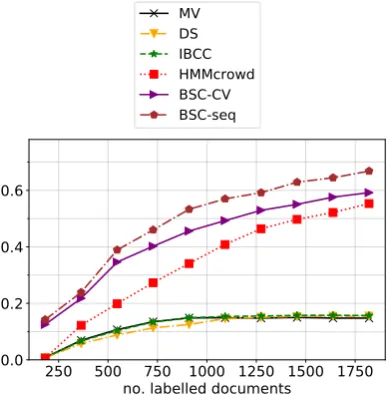
250 500 750 1000 1250 1500 1750 no. labelled documents
0.0 0.2 0.4 0.6
F1 score
MV DS IBCC HMMcrowd BSC-CV BSC-seq
250 500 750 1000 1250 1500 1750 no. labelled documents
0.0 0.2 0.4 0.6
F1 score
[image:9.595.83.279.65.263.2]MV DS IBCC HMMcrowd BSC-CV BSC-seq
Figure 2: F1 scores for active learning simulations on NER using least-confidence uncertainty sampling.
uncertainty in the model parameters when esti-mating confidence, hence can be used to choose data points that rapidly improve the model itself. Sequential models such as BSC can also account for dependencies between sequence labels when estimating confidence.
Input: A randominitial setof training labels, the same for all methods.
1 Set training setc=initial set
whiletraining set size< max no labelsdo 2 Train model onc
3 For each documentn, compute
LCn= 1−p(t∗n|c), wheret∗nis the probability of the most likely sequence of labels forn.
4 Obtain annotations forbatch size
documents with the highest values ofLC (least confidence), and add them toc
end
Algorithm 2: Active learning simulation using least-confidence sampling.
Figure2 plots the mean F1 scores over ten re-peats of the active learning simulation on the NER dataset (for clarity, we only plot key methods). When the number of iterations is very small, nei-ther IBCC nor DS are able to outperform ma-jority vote, and only produce a very small ben-efit as the number of labels grows. This high-lights the need for a sequential model such as BSC or HMM-crowd for effective active learning with small numbers of labels. IBCC learns slightly
quicker than DS, while BSC-CV clearly outper-forms HMM-crowd: we believe this difference is due to the Bayesian treatment of IBCC and BSC, which means they are better able to estimate confi-dence than DS and HMM-crowd, which use max-imum likelihood and maxmax-imum a posteriori infer-ence. BSC-seq produces the best overall perfor-mance, and the gap grows as the number of labels increases, since more data is required to learn the more complex annotator model.
7 Conclusions
We proposed BSC, a novel Bayesian approach to aggregating sequence labels that can be combined with several different models of annotator noise and bias. To model the effect of dependencies between labels on annotator noise and bias, we introduced the seq annotator model. Our results demonstrated the benefits of BSC over established non-sequential methods, such as MACE, Dawid-Skene (DS), and IBCC. We also showed the ad-vantages of a Bayesian approach for active learn-ing, and that the combination ofBSCwith theseq annotator model improves the state-of-the-art over HMM-crowd on three NLP tasks with different types of span annotations.
In future work, we plan to adapt active learning methods for easy deployment on crowdsourcing platforms, and to investigate techniques for auto-matically selecting good hyperparameters without recourse to a development set, which is often un-available at the start of a crowdsourcing process.
Acknowledgments
This work was supported by the German Research Foundation through the German-Israeli Project Cooperation (DIP, grant DA 1600/1-1 and grant GU 798/17-1), and by the German Research Foun-dation (DFG) as part of the QA-EduInf project (grant GU 798/18-1 and grant RI 803/12-1). We would like to thank all of those who developed the datasets used in this work.
References
Hagai Attias. 2000. A variational Bayesian framework for graphical models. InAdvances in Neural Infor-mation Processing Systems 12, pages 209–215. MIT Press.
the answers: a Bayesian graphical model for adap-tive crowdsourcing and aptitude testing. In Proceed-ings of the 29th International Coference on Interna-tional Conference on Machine Learning, pages 819– 826. Omnipress.
Christopher. M. Bishop. 2006.Pattern recognition and machine learning, 4th edition. Information Science and Statistics. Springer.
David M. Blei, Andrew Y. Ng, and Michael I. Jordan. 2003. Latent Dirichlet allocation. The Journal of Machine Learning Research, 3:993–1022.
Alexander Philip Dawid and Allan M. Skene. 1979.
Maximum likelihood estimation of observer error-rates using the EM algorithm. Journal of the Royal Statistical Society. Series C (Applied Statis-tics), 28(1):20–28.
Thomas G Dietterich. 2000.Ensemble methods in Ma-chine Learning. InMultiple classifier systems, pages 1–15. Springer.
Pinar Donmez, Jaime Carbonell, and Jeff Schneider. 2010.A probabilistic framework to learn from mul-tiple annotators with time-varying accuracy. In Pro-ceedings of the 2010 SIAM International Conference on Data Mining, pages 826–837. SIAM.
Paul Felt, Eric K. Ringger, and Kevin D. Seppi. 2016.
Semantic annotation aggregation with conditional crowdsourcing models and word embeddings. In In-ternational Conference on Computational Linguis-tics, pages 1787–1796.
Zoubin Ghahramani. 2001. An introduction to hidden markov models and Bayesian networks. Interna-tional Journal of Pattern Recognition and Artificial Intelligence, 15(01):9–42.
Dirk Hovy, Taylor Berg-Kirkpatrick, Ashish Vaswani, and Eduard H Hovy. 2013. Learning whom to trust with MACE.InHLT-NAACL, pages 1120–1130.
Hyun-chul Kim and Zoubin Ghahramani. 2012.
Bayesian classifier combination. In International Conference on Artificial Intelligence and Statistics, pages 619–627.
Guillaume Lample, Miguel Ballesteros, Sandeep Sub-ramanian, Kazuya Kawakami, and Chris Dyer. 2016.
Neural architectures for named entity recognition. InProceedings of NAACL-HLT, pages 260–270.
Xuezhe Ma and Eduard Hovy. 2016. End-to-end sequence labeling via bi-directional LSTM-CNNs-CRF. InProceedings of the 54th Annual Meeting of the Association for Computational Linguistics (Vol-ume 1: Long Papers), volume 1, pages 1064–1074.
Pablo G. Moreno, Yee Whye Teh, and Fernando Perez-Cruz. 2015. Bayesian nonparametric crowd-sourcing. Journal of Machine Learning Research, 16:1607–1627.
An T Nguyen, Byron C Wallace, Junyi Jessy Li, Ani Nenkova, and Matthew Lease. 2017. Aggregating and predicting sequence labels from crowd anno-tations. In Proceedings of the conference. Associ-ation for ComputAssoci-ational Linguistics. Meeting, vol-ume 2017, page 299. NIH Public Access.
Silviu Paun, Bob Carpenter, Jon Chamberlain, Dirk Hovy, Udo Kruschwitz, and Massimo Poesio. 2018.
Comparing Bayesian models of annotation. Trans-actions of the Association for Computational Lin-guistics, 6:571–585.
Vikas. C. Raykar, Shipeng Yu, Linda H. Zhao, Ger-ardo Hermosillo. Valadez, Charles Florin, Luca Bo-goni, and Linda Moy. 2010. Learning from crowds.
Journal of Machine Learning Research, 11:1297– 1322.
Filipe Rodrigues, Francisco Pereira, and Bernardete Ribeiro. 2013. Learning from multiple annotators: distinguishing good from random labelers. Pattern Recognition Letters, 34(12):1428–1436.
Filipe Rodrigues, Francisco Pereira, and Bernardete Ribeiro. 2014. Sequence labeling with multiple an-notators. Machine learning, 95(2):165–181.
Burr Settles. 2010. Active learning literature survey.
Computer Sciences Technical Report 1648, Univer-sity of Wisconsin-Madison, 52(55-66):11.
Burr Settles and Mark Craven. 2008.An analysis of ac-tive learning strategies for sequence labeling tasks. InProceedings of the conference on empirical meth-ods in natural language processing, pages 1070– 1079. Association for Computational Linguistics.
Aashish Sheshadri and Matthew Lease. 2013.
SQUARE: A benchmark for research on computing crowd consensus. In First AAAI Conference on Human Computation and Crowdsourcing.
Edwin Simpson, Stephen J. Roberts, Ioannis Psorakis, and Arfon Smith. 2013. Dynamic Bayesian combi-nation of multiple imperfect classifiers. Intelligent Systems Reference Library series, Decision Making with Imperfect Decision Makers:1–35.
Nitish Srivastava, Geoffrey Hinton, Alex Krizhevsky, Ilya Sutskever, and Ruslan Salakhutdinov. 2014.
Dropout: a simple way to prevent neural networks from overfitting. The Journal of Machine Learning Research, 15(1):1929–1958.
Erik F Tjong Kim Sang and Fien De Meulder. 2003. Introduction to the CoNLL-2003 shared task: Language-independent named entity recognition. In
Proceedings of the seventh conference on Natural language learning at HLT-NAACL 2003-Volume 4, pages 142–147. Association for Computational Lin-guistics.
Dietrich Trautmann, Johannes Daxenberger, Christian Stab, Hinrich Sch¨utze, and Iryna Gurevych. 2019.
Robust argument unit recognition and classification.
Matteo Venanzi, John Guiver, Gabriella Kazai, Pushmeet Kohli, and Milad Shokouhi. 2014.
Community-based Bayesian aggregation models for crowdsourcing. In23rd international conference on World wide web, pages 155–164.
Matteo Venanzi, John Guiver, Pushmeet Kohli, and Nicholas R Jennings. 2016. Time-sensitive Bayesian information aggregation for crowdsourc-ing systems. Journal of Artificial Intelligence Re-search, 56:517–545.
Andrew Viterbi. 1967. Error bounds for convolutional codes and an asymptotically optimum decoding al-gorithm.IEEE transactions on Information Theory, 13(2):260–269.
Jacob Whitehill, Ting-fan Wu, Jacob Bergsma, Javier R Movellan, and Paul L Ruvolo. 2009. Whose vote should count more: Optimal integration of labels from labelers of unknown expertise. InAdvances in neural information processing systems, pages 2035– 2043.
Hui Yuan Xiong, Yoseph Barash, and Brendan J Frey. 2011. Bayesian prediction of tissue-regulated splic-ing ussplic-ing rna sequence and cellular context. Bioin-formatics, 27(18):2554–2562.
Harry Zhang. 2004. The optimality of na¨ıve Bayes. In Proceedings of the Seventeenth International Florida Artificial Intelligence Research Society Conference, FLAIRS 2004. AAAI Press.
A Discussion of Variational Approximation
In Equation 12, each subset of latent variables has a variational factor of the form lnq(z) = E[lnp(z|c,¬z)], where ¬z contains all the other latent variables excludingz. We perform approx-imate inference by using coordinate ascent to up-date each variational factor, q(z), in turn, taking expectations with respect to the current estimates of the other variational factors. Each iteration re-duces the KL-divergence between the true and ap-proximate posteriors of Equation 12, and hence optimises a lower bound on the log marginal like-lihood, also called the evidence lower bound or ELBO (Bishop,2006;Attias,2000).
Conjugate distributions: The prior distribu-tions chosen for our generative model are conju-gate to the distributions over the latent variables and model parameters, meaning that eachq(z)is the same type of distribution as the corresponding prior distribution defined in Section 4. The param-eters of each variational distribution are computed in terms of expectations over the other subsets of variables.
B Update Equations for the Forward-Backward Algorithm
For the true labels,t, the variational factor is:
lnq(tn) = N X
n=1 Ln X
τ=1 K X
k=1
ElnA(k)
tn,τ, c(k)n,τ, c (k) n,τ−1
+ElnTtn,τ−1,tn,τ+ const. (21)
The forward-backward algorithm consists of two passes. Theforward passfor each document, n, starts fromτ = 1and computes:
lnrn,τ,j− = ln J X
ι=1 n
r−n,τ−1,ιeElnTι,j o
+lln,τ(j),
lln,τ(j) = K X
k=1
ElnA(k)
j, c(k)n,τ, c(k)n,τ−1
(22)
where rn,0,ι− = 1 where ι =‘O’ and 0 other-wise. The backwards pass starts from τ = Ln and scrolls backwards, computing:
lnλn,Ln,j = 0, lnλn,τ,j = ln J X
ι=1 exp
lnλi,τ+1,ι+ElnTj,ι+lln,τ+1(ι) . (23)
By applying Bayes’ rule, we arrive at rn,τ,j and sn,τ,j,ι:
rn,τ,j =
rn,τ,j− λn,τ,j
PJ
j0=1r−n,τ,j0λn,τ,j0
(24)
sn,τ,j,ι=
˜ sn,τ,j,ι
PJ
j0=1
PJ
ι0=1s˜n,τ,j0,ι0
(25)
˜
sn,τ,j,ι=r−n,τ−1,jλn,τ,ιexp{ElnTj,ι+lln,τ(ι)}.
Each row of the transition matrix has the factor:
lnq(Tj) = ln Dir ([Nj,ι+γj,ι,∀ι∈ {1, .., J}]), (26)
where Nj,ι = PNn=1PLτ=1n sn,τ,j,ι is the ex-pected number of times that labelιfollows labelj. The forward-backward algorithm requires expec-tations of lnT that can be computed using stan-dard equations for a Dirichlet distribution:
ElnTj,ι = Ψ(Nj,ι+γj,ι)−Ψ
J X
ι=1
(Nj,ι+γj,ι) !
,
(27)
BSC-seq,
previous label = I: true label I O B
worker label IO
B0 1
Cluster 0
I O B IOB 0
1
Cluster 1
I O B IOB 0
1
Cluster 2
I O B IOB 0
1
Cluster 3
I O B IOB 0
1
Cluster 4
BSC-seq,
previous label = O: true label I O B
worker label IO
B0 1
Cluster 0
I O B IOB 0
1
Cluster 1
I O B IOB 0
1
Cluster 2
I O B IOB 0
1
Cluster 3
I O B IOB 0
1
Cluster 4
BSC-seq,
previous label = B: true label I O B
worker label IO
B0 1
Cluster 0
I O B IOB 0
1
Cluster 1
I O B IOB 0
1
Cluster 2
I O B IOB 0
1
Cluster 3
I O B IOB 0
[image:12.595.76.526.62.342.2]1
Cluster 4
Figure 3: Clusters of annotators in PICO represented by the mean confusion matrices from BSC-seq. Heights of bars indicate likelihood of a worker (or annotator) label given the true label.
The variational factor for each annotator model is a distribution over its parameters, which differs between models. Forseq, the variational factor is:
lnqA(k)= J X
j=1 J X
l=1
DirhN(k)j,l,m∀m∈ {1, .., J}i
Nj,l,m(k) =α(k)j,l,m+ N X
n=1 Ln X
τ=1
rn,τ,jδl,c(k)
n,τ−1
δ
m,c(n,τk), (28)
whereδ is the Kronecker delta. ForCM,MACE, CVandacc, the factors follow a similar pattern of summing pseudo-counts of correct and incorrect answers.
C Visualising Annotator Models
[image:12.595.72.293.455.531.2]