Proceedings of the 2019 Conference on Empirical Methods in Natural Language Processing 3400
Autoregressive Text Generation Beyond Feedback Loops
Florian Schmidt
Department of Computer Science ETH Z¨urich
Stephan Mandt
Department of Computer Science University of California, Irvine
Thomas Hofmann
Department of Computer Science ETH Z¨urich
Abstract
Autoregressive state transitions, where predic-tions are conditioned on past predicpredic-tions, are the predominant choice for both determinis-tic and stochasdeterminis-tic sequential models. How-ever, autoregressive feedback exposes the evo-lution of the hidden state trajectory to po-tential biases from well-known train-test dis-crepancies. In this paper, we combine a la-tent state space model with a CRF observa-tion model. We argue that such autoregres-sive observation models form an interesting middle ground that expresses local correla-tions on the word level but keeps the state evo-lution non-autoregressive. On unconditional sentence generation we show performance im-provements compared to RNN and GAN base-lines while avoiding some prototypical failure modes of autoregressive models.1
1 Introduction
Sequential autoregressive models express pre-dictions of observations based on past predic-tions. They are the predominant architecture for text generation in a maximum likelihood setup (Graves,2013;Sutskever et al.,2014) and are used in machine translation (Bahdanau et al., 2015;
Vaswani et al.,2017), summarization (Rush et al.,
2015), and dialogue systems (Serban et al.,2016). An immediate consequence of combining au-toregressive modeling and maximum likelihood training is that past observations enter the loss functions as ground-truth, not predicted observa-tions (Goodfellow et al.,2016). This discrepancy is often summarized as teacher-forcing and the bias it implies is referred to asexposure-bias( Ran-zato et al.,2016;Goyal et al.,2016).
1Code and generated sentences available athttps://
github.com/schmiflo/crf-generation
The standard methodology to turn a sequen-tial model into an autoregressive one is to intro-duce afeedback loop, where one provides the last predicted token as a feature to the computation of the next state (Graves, 2013). The ground-truth observations become effectively input fea-tures for the evolution of the hidden state trajec-tory at training time. Several attempts have been made to introduce robustness with respect to the model’s predictions by leaving the maximum like-lihood framework, either implicitly (Bengio et al.,
2015;Bowman et al., 2016) or explicitly (Goyal et al., 2016; Leblond et al., 2018). Neverthe-less, the same feedback mechanisms have been adopted in latent sequential models where they obfuscate the true stochasticity of transitions dur-ing traindur-ing. Non-autoregressive sequence mod-els have recently regained attention for uncondi-tional (Schmidt and Hofmann, 2018;M. Ziegler and M. Rush, 2019) and conditional (Lee et al.,
2018) generation.
We argue that there is an interesting interme-diate regime between feedback-driven autoregres-sive models and completely non-autoregresautoregres-sive models, namely modeling temporal correlations as part of theobservation model. We propose a neu-ral CRF observation model that leverages word-embeddings to explain local word correlations in a global sequence score. We show how training and generation can be performed efficiently. The result is an autoregressive model that keeps the hidden state evolution less affected by observation noise while generating coherent word sequences.
2 Related Work
label bias, a shortcoming of locally normalized observation models. They have been applied and integrated into neural-network architectures (Ma and Hovy,2016;Huang et al.,2017) in various se-quence labeling tasks (Goldman and Goldberger,
2017) where the observation space exhibits small cardinality (typically tens to hundreds).
The importance of global normalization for se-quence generation has only lately been empha-sized, most notably byWiseman and Rush(2016) for conditional generation in a learning-as-search-optimization framework and by (Andor et al.,
2016) for parsing.
Word-embeddings have been reported as excel-lent dense representations of sparse co-occurrence statistics within several learning frameworks (Mikolov et al., 2013; Pennington et al., 2014). Using embeddings in pairwise potentials has been proposed byGoldman and Goldberger(2017), but they do not compute the true log-likelihood during training as we do. Similar techniques have been applied for various message passing schemata (Kim et al.,2017;Domke,2013).
Local correlations such as our pairwise poten-tials have been used by (Noraset et al.,2018), yet as an auxiliary loss and not for model design.
Other approaches to tackle teacher-forcing have been proposed in an adversarial setting (Goyal et al., 2016), in search based optimiza-tion (Leblond et al.,2018) and in a reinforcement learning setting (Rennie et al.,2016).
3 Model
Latent sequential models for text generation typi-cally consist of two parts: A mechanism for gener-ating a latent hidden state trajectoryh=h1:T, and
an observation model. The latter predicts the data
w = w1:T given the latent states. The most
sim-ple dependency structure for such a model is that of an Hidden Markov Model, which breaks into transitionsp(ht|ht−1)and observationsp(wt|ht).
In contrast, models withautoregressive transitions
factorize as
p(w,h) =
T
Y
t=1
p(wt|ht)p(ht|ht−1, wt−1). (1)
The result is a next-state distribution with depen-dencies identical to deterministic RNN transitions ht = F(ht−1, wt−1) and indeed similar neural
networks can be used to parametrize a simple, e.g., Gaussian distribution (Fraccaro et al.,2016).
As a negative consequence, we inherit teacher-forcing. This comes with aforementioned biases and also conflicts with our notion of uncertainty inp(ht|ht−1, wt−1) which during training solely
depends on the continuous parameters (i.e. a mean and a variance), but is greatly affected by the dis-crete sampling noise inwt−1at test time.
Autoregressive observation model We con-sider an alternative to autoregressive feedback mechanisms such as (1), where predictions are di-rectly injected into states. We write
p(w,h) =p(w|h)
T
Y
t=1
p(ht|ht−1) (2)
assuming only Markovian transitions and focus on finding a powerful observation model instead. Crucially, since the state space model is not af-fected by previous outputs, word coherence may be lost when simply factorizing as in p(w|h) =
Q
tp(wt|ht), i.e. with independent soft-max
fac-torsp(wt|ht)∝expψ(wt,ht)whereψ(wt,ht) =
x(wt)>ht. However, a natural extension can be
found by reformulating local normalization as a form of global normalization without correlations across time
p(w|h) =
T
Y
t=1
expψ(wt,ht)
P
w0
texpψ(w
0
t,ht)
(3)
= PexpS(w,h)
w0expS(w0,h)
(4)
where S = PT
t=1ψ(wt,ht) contains no
depen-dencies betweenwtandwt0 fort6=t0. As soon as
we add word-correlations to S, we obtain a truly global observation model that cannot be expressed in the form of (3).
3.1 CRF Observation Model
Equation (4) describes a conditional random field (CRF) with an energy functionS(Sha and Pereira,
2003). We consider up to pairwise interactions be-tween consecutive words
S(w;h) =
T
X
t=1
ψ(wt;ht)+ψ(wt−1, wt;ht−1:t)(5)
The potentialsψreflect the independence assump-tions among w and determine the complexity of the normalizerZ =P
w0expS(w0). Fortunately,
w1 w1 w1 w1
w2 w2 w2 w2
w3 w3 w3 w3
h1 h2 h3 h4
p(w) =
T
Y
t=1
expψ(wt;ht)
P
wt0expψ(w0t;ht)
w1 w1 w1 w1
w2 w2 w2 w2
w3 w3 w3 w3
h1 h2 h3 h4
p(w) =Pexpψ(w;h)
w0expψ(w0;h)
w1
w2
w3
w1
w2
w3
w1
w2
w3
w1
w2
w3 h(w(1)1:T)
h(w(2)1:T)
h(w(3)1:T) . . .
h(w(1:|VT|T))
p(w) =Pexpψ(h(w))
[image:3.595.79.519.66.181.2]w0expψ(h(w0))
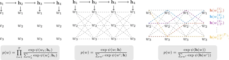
Figure 1: Schematic comparison of differently normalized architectures. We sketch trellis diagrams for V = {w1, w2, w3}andT = 4. Dashed lines indicate autoregressive dependencies in the log-likelihood computation.
Left: Standard RNN with soft-max observations. Since the model is locally normalized, the trellis diagram does not unfold across time-steps. Middle: Our proposed CRF model. The potentials only span across pairs, but the normalization is global and can be computed exactly and efficiently. Right: An intractable globally normalized model in which fully-connected potentialsψ(h(w))are obtained from an RNN. Computing a singlep(w)would require running the RNN|V|T times. We highlight four runs for illustration.
Two properties set our model apart from feedback-driven autoregressive models. First, al-though ψ captures only pairwise interactions, a statehtwill not only affect future observations but
also allpast observations through the global cou-pling. Second, our model implicitly considersall
possible sequenceswalso at training time due to the global normalizerZ.
3.2 Sampling
Given a trained model, we can perform ances-tral sampling via h ∼ p(h) and w ∼ p(w|h). However, CRFs are undirected graphical models not designed with generation in mind and there-fore we first need to derive ancestral sampling for p(w|h). We can always write p(w|h) =
Q
tp(wt|w1:t−1,h)and find the factors
p(wt|w1:t−1,h) =eψ(wt−1,wt)+ψ(wt)
βt+1(wt)
βt(wt−1)
(6)
where
βt(wt−1) =
X
wt
eψ(wt−1,wt)+ψ(wt)β
t+1(wt) (7)
with special casesβ1(w0) = 1andβT+1(wT) =
Zare the backwards probabilities we anyway need to compute for (4). Not surprisingly, multiplying (6) for t = 1 :T lets all β terms cancel except for 1/Z and we recover (4). However, this form is more amendable to sampling2and reveals an in-teresting property of globally normalized models: While the chain rule always allows to write such
2In fact, one can train on (6) instead of (4). However, in our experiments we found the latter global normalization to be much more stable numerically.
models autoregressively, we must expect a factor – hereβt+1(wt)– that implicitly marginalizes out
future observations to assess compatibility with a specific next wordwt. Tractability of this factor
is key to obtain a tractable model and is traded for expressiveness. While locally normalized models are on one end of the spectrum, a globally nor-malized with fully-connected potentialsψ(h(w))
is on the other end. Such models employ an RNN ineachpotential to obtain an un-normalized score
ψfrom stateshand have been investigated in con-ditional generation where argmax-decoding rather than sampling is requried (Wiseman and Rush,
2016). Figure1shows the dependencies of the two extremes with our model in the middle.
3.3 Embedding-based Local Correlations
Often pairwise potentials can be parametrized di-rectly, i.e. asψ(wi, wj) = Aij for some
param-eter matrix A ∈ RV×V. However, in our setting
this is problematic for two reasons. First,|V|2
pa-rameters are impractical in terms of model size for most vocabularies. Second, computations involv-ingAare central to the complexity of computing log-likelihood during training. Namely, to com-pute the normalizerZ, we need to compute allβ
quantities in (7). Identifyingβt(wt−1) as a |V|
-dimensional vectorβt, we can write the
summa-tion in (7) as a matrix-vector product
βt=T(otβt+1) (8)
where is an element-wise product, ot are the
unary potentials ψ(wt) written as a vector and
To overcome the above shortcomings, we pro-pose to factorizeTas
T=X>S(ht−1,ht)Y (9)
into context-independent d-dimensional embed-dings X,Y ∈ Rd×|V| and a context-dependent
d ×d interaction matrix computed by a neural network S : Rd
0
×Rd 0
→ Rd×d. This reduces
the memory requirement toO(d|V|)and compute time to O(d|V|T), which is comparable to com-puting standard soft-max logits. As an additional benefit we can initializeXandYwith pre-trained word-embeddings, a technique often reported to improve convergence. SineAdoes not have more structure than being strictly positive element-wise, it is sufficient to use strictly positive activation functions around the layers in (8) to obtain a valid factorization.
3.4 Training
As is standard for latent sequential models, we use variational inference for training (Blei et al.,2017;
Zhang et al.,2018). We introduce a parametrized approximate inference modelq(h|w)to maximize the evidence lower bound (ELBO) for a sam-pled trajectory instead of maximizing the marginal across all trajectories:
logp(w) =
Z
p(w,h)dh (10)
≥Eq
logp(w|h) + log p(h)
q(h|w)
(11)
The first term of (11) measures reconstruction while the second measures the discrepancy be-tween the trajectories implied by the inference model q and the generative model p. The ex-act form ofp(h)depends on its factorization and if it is autoregressive but for us simply p(h) =
Q
tp(ht|ht−1), which casts us as an
autoregres-sive extension ofSchmidt and Hofmann(2018).
Inference model Like (Fraccaro et al., 2016), we chooseqto factorize as the true posterior
q(h|w) =
T
Y
t=1
q(ht|ht−1, wt:T) (12)
where w1:T is encoded using an RNN running
backwards in time to parameterize mean and vari-ance of a Gaussian for q(ht|ht−1, wt:T). For
optimization we follow existing work (Fraccaro
et al., 2016; Goyal et al., 2017) and use the re-parametrization trick (Rezende et al., 2014;
Kingma et al.,2016) to perform a stochastic gra-dient step on (11) with Adam (Kingma and Ba,
2014) using a single trajectory.
4 Experiments
Exposure-bias can be summarized as over-confident conditioning on “pseudo” predictions during training. The strength of the bias depends on the informativeness of such predictions, which in turn depends on the remaining context provided. We test our proposed method onunconditional
generation which does not provide context such as a source sentence to narrow down possible outputs a priori. Hence, potential biases are more pro-nounced and generation is isolated from effects in-duced by i.e. a translation or summarization task.
Setup Unconditional generation is still consid-ered a challenging task for both, GANs and la-tent stochastic models, (Fedus et al., 2018) and standard RNNs form a very competitive baseline (Semeniuta et al., 2018). To obtain a homoge-neous text dataset of low complexity we extract the plain text (text and hypothesis) from the Standard SNLI dataset (Bowman et al., 2015) (For details and samples see AppendixA).
Baselines We compare against a GRU (an LSTM performed on par) standard RNN of match-ing state size denoted DRNN. We also include SeqGAN3 (Yu et al., 2017), a popular GAN ar-chitecture for unconditional generation. Further, we restrict our model to unary potentials to ob-tain a non-autoregressive state space model similar to that of Schmidt and Hofmann(2018), denoted SSM. Finally, 2-GRAM is a bi-gram language model and ORACLE is held-out data, which rep-resents the gold-standard for unconditional gener-ation.
Parameterization We use 16-dimensional la-tent states, pre-train 100-dimensional GloVe em-beddings and use word and context vectors for Y and X. For S we found a diagonal matrix to perform best. In this case, the symmetry of T is broken by larger unary potentials. While we find larger word embedding dimensionality to improve performance, the model does not benefit from more latent dimensions as an RNN does from
hidden dimensions, a known issue of deep latent variable models (Schmidt and Hofmann, 2018;
M. Ziegler and M. Rush,2019).
4.1 Qualitative Results
Table 1 shows selected output generated by our model (See AppendixBfor more output). While
a dog runs .
the children are alone . the man is being beaten .
the man is inside working onstage . the dog is outside with his girlfriend .
two dogs going swimming in an open-air festival . a young lady wearing a pink shirt is studying .
Table 1: Output of our model of different length.
many of our sentences are grammatical and mimic those of the dataset we note that the corpus is not large enough to learn common sense and all models including the baselines sometimes gener-ate output such astwo men are burning snow.
4.2 Quantitative Results
Perplexity under external language models is the standard metric to evaluate unconditional output (Fedus et al., 2018) and we use Kneser-Ney-smoothed models up to4 n = 3estimated on the training data using SRILM (Stolcke,2002).
In addition, we propose to estimate some impor-tant aggregate statistics easily verifiable against the real data. We choose lengthland percentage of unique sentencesρUNI to assess diversity and per-centage of token repetitionsρREPto adress a failure mode often found in generative models (Tu et al.,
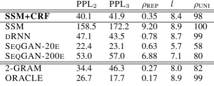
2016). Table2shows the results.
PPL2 PPL3 ρREP l ρUNI
SSM+CRF 40.1 41.9 0.35 8.4 98
SSM 158.5 172.2 9.20 8.9 100
DRNN 47.1 43.5 0.78 8.7 99
SEQGAN-20E 22.4 23.1 0.63 5.7 58 SEQGAN-200E 53.0 57.0 6.88 7.1 80
2-GRAM 34.4 46.3 0.27 8.0 82
[image:5.595.73.288.560.647.2]ORACLE 26.7 17.7 0.17 8.9 99
Table 2: Our modelSSM+CRFevaluated against the baselines on 100K generated sentences each: Perplex-ity of output under external language model PPLn, per-centage of repeated tokens per sentenceρREP, lengthl,
and percentage of unique sentencesρUNI. All statistics
should be compared to ORACLE, a held-out data split.
4We find that the data is too sparse to train 4-gram lan-guage models as measured on a test-set.
5 Discussion and Future Work
In terms of perplexity our model clearly improves over SSM, outperforms DRNN as measured by bigram statistics, and is on par with it in terms of trigram statistics. Of course, 2-GRAM excels in terms of bigram statistics, yet falls behind on longer statistics. This confirms that our model can learn beyond pairwise interactions through the la-tent chain. In addition, through our explicit model of pairwise interaction we obtain repetitionsρREP significantly closer to the real data distribution.
For SEQGAN we report after 20 epochs (as used by the authors) and 200 epochs. We observe in general shorter output with more repetition (i.e. of wordsare, isandup) and note that depending on training time the stellar fluency is traded with a significant bias on lengthland very poor diversity
ρUNI, a tendency also observed byXu et al.(2018) and possibly related to the choice of temperature parameter (Caccia et al.,2018). While it is not our goal to provide a deeper analysis of GANs here, the example shows how unconditional generation can reveal tradeoffs not present in a conditional setting.
Future Work We have shown that autoregres-sive predictions expressed in the observation model instead of hidden states deliver better re-sults on a simple corpus. In particular, mistakes at the bigram-level, such as repetitions, are avoided and we suspect that more densely connected CRFs allow to extend these promising results to more complex patterns found in more complex corpora. In future work we plan to investigate if CRF vari-ants such as (Belanger et al.,2017) or (Kr¨ahenb¨uhl and Koltun,2012) can be adapted to allow efficient sampling and to scale to word vocabulary sizes.
6 Conclusion
References
Daniel Andor, Chris Alberti, David Weiss, Aliaksei Severyn, Alessandro Presta, Kuzman Ganchev, Slav Petrov, and Michael Collins. 2016. Globally nor-malized transition-based neural networks. CoRR, abs/1603.06042.
Dzmitry Bahdanau, Kyunghyun Cho, and Yoshua Ben-gio. 2015. Neural machine translation by jointly learning to align and translate. InICLR.
David Belanger, Bishan Yang, and Andrew McCallum. 2017. End-to-end learning for structured prediction energy networks. InICML.
Samy Bengio, Oriol Vinyals, Navdeep Jaitly, and Noam Shazeer. 2015. Scheduled sampling for se-quence prediction with recurrent neural networks. InNIPS.
David M Blei, Alp Kucukelbir, and Jon D McAuliffe. 2017. Variational inference: A review for statisti-cians. Journal of the American Statistical Associa-tion.
Samuel R. Bowman, Gabor Angeli, Christopher Potts, and Christopher D. Manning. 2015. A large anno-tated corpus for learning natural language inference. InEMNLP.
Samuel R. Bowman, Luke Vilnis, Oriol Vinyals, An-drew M. Dai, Rafal J´ozefowicz, and Samy Ben-gio. 2016. Generating sentences from a continuous space. InACL.
Massimo Caccia, Lucas Caccia, William Fedus, Hugo Larochelle, Joelle Pineau, and Laurent Charlin. 2018. Language gans falling short. CoRR, abs/1811.02549.
Justin Domke. 2013.Learning graphical model param-eters with approximate marginal inference. InIEEE Transactions on Pattern Analysis and Machine In-telligence.
William Fedus, Ian J. Goodfellow, and Andrew M. Dai. 2018. Maskgan: Better text generation via filling in the . InICLR.
Marco Fraccaro, Søren Kaae Sø nderby, Ulrich Paquet, and Ole Winther. 2016. Sequential neural models with stochastic layers. InNIPS.
Eran Goldman and Jacob Goldberger. 2017. Struc-tured image classification from conditional random field with deep class embedding. arXiv preprint arXiv:1705.07420.
Ian Goodfellow, Yoshua Bengio, and Aaron Courville. 2016.Deep Learning. MIT Press.
Anirudh Goyal, Alex Lamb, Ying Zhang, Saizheng Zhang, Aaron C. Courville, and Yoshua Bengio. 2016. Professor forcing: A new algorithm for train-ing recurrent networks. InNIPS.
Anirudh Goyal, Alessandro Sordoni, Marc-Alexandre Cˆot´e, Nan Rosemary Ke, and Yoshua Bengio. 2017.
Z-forcing: Training stochastic recurrent networks. InNIPS.
Alex Graves. 2013. Generating sequences with recurrent neural networks. arXiv preprint arXiv:1308.0850.
Zhiheng Huang, Wei Xu, and Kai Yu. 2017. Bidi-rectional LSTM-CRF models for sequence tagging. InFirst Workshop on Subword and Character Level Models in NLP.
Yoon Kim, Carl Denton, Luong Hoang, and Alexan-der M. Rush. 2017. Structured attention networks. InICLR.
Diederik P. Kingma and Jimmy Ba. 2014. Adam: A method for stochastic optimization. InICLR.
Diederik P. Kingma, Tim Salimans, and Max Welling. 2016. Improving variational inference with inverse autoregressive flow. InNIPS.
Philipp Kr¨ahenb¨uhl and Vladlen Koltun. 2012. Effi-cient inference in fully connected crfs with gaussian edge potentials. InNIPS.
R´emi Leblond, Jean-Baptiste Alayrac, Anton Osokin, and Simon Lacoste-Julien. 2018. SEARNN: train-ing rnns with global-local losses. InICLR.
Jason Lee, Elman Mansimov, and Kyunghyun Cho. 2018. Deterministic non-autoregressive neural sequence modeling by iterative refinement. In
EMNLP.
Zachary M. Ziegler and Alexander M. Rush. 2019. La-tent normalizing flows for discrete sequences.arXiv preprint arXiv:1901.10548.
Xuezhe Ma and Eduard H. Hovy. 2016.End-to-end se-quence labeling via bi-directional lstm-cnns-crf. In
ACL.
Tomas Mikolov, Ilya Sutskever, Kai Chen, Greg S Cor-rado, and Jeff Dean. 2013. Distributed representa-tions of words and phrases and their compositional-ity. InNIPS.
Thanapon Noraset, David Demeter, and Doug Downey. 2018. Controlling global statistics in recurrent neu-ral network text generation.
Jeffrey Pennington, Richard Socher, and Christo-pher D. Manning. 2014. Glove: Global vectors for word representation. InEMNLP.
Marc’Aurelio Ranzato, Sumit Chopra, Michael Auli, and Wojciech Zaremba. 2016. Sequence level train-ing with recurrent neural networks. InICLR.
Danilo Jimenez Rezende, Shakir Mohamed, and Daan Wierstra. 2014. Stochastic back-propagation and variational inference in deep latent gaussian models. InICML.
Alexander M. Rush, Sumit Chopra, and Jason Weston. 2015. A neural attention model for abstractive sen-tence summarization. InEMNLP.
Florian Schmidt and Thomas Hofmann. 2018. Deep state space models for unconditional word genera-tion. InNeurIPS.
Stanislau Semeniuta, Aliaksei Severyn, and Sylvain Gelly. 2018. On accurate evaluation of gans for lan-guage generation. InICML workshop on Theoreti-cal Foundations and Applications of Deep Genera-tive Models.
Iulian Vlad Serban, Alessandro Sordoni, Yoshua Ben-gio, Aaron C Courville, and Joelle Pineau. 2016.
Building end-to-end dialogue systems using gener-ative hierarchical neural network models. InAAAI.
Fei Sha and Fernando Pereira. 2003. Shallow parsing with conditional random fields. InNAACL.
Andreas Stolcke. 2002.Srilm – an extensible language modeling toolkit. InICSLP.
Ilya Sutskever, Oriol Vinyals, and Quoc V. Le. 2014.
Sequence to sequence learning with neural net-works. InNIPS.
Zhaopeng Tu, Yang Liu, Lifeng Shang, Xiaohua Liu, and Hang Li. 2016.Neural machine translation with reconstruction.CoRR, abs/1611.01874.
Ashish Vaswani, Noam Shazeer, Niki Parmar, Jakob Uszkoreit, Llion Jones, Aidan N. Gomez, Lukasz Kaiser, and Illia Polosukhin. 2017. Attention is all you need. InNIPS.
Sam Wiseman and Alexander M. Rush. 2016.
Sequence-to-sequence learning as beam-search op-timization. InEMNLP.
Jingjing Xu, Xu Sun, Xuancheng Ren, Junyang Lin, Bingzhen Wei, and Wei Li. 2018. DP-GAN: diversity-promoting generative adversarial network for generating informative and diversified text. In
EMNLP.
Lantao Yu, Weinan Zhang, Jun Wang, and Yong Yu. 2017.Seqgan: Sequence generative adversarial nets with policy gradient. InAAAI.