Hierarchical CVAE for Fine-Grained Hate Speech Classification
Jing Qian, Mai ElSherief, Elizabeth Belding, William Yang Wang Department of Computer Science
University of California, Santa Barbara Santa Barbara, CA 93106 USA
{jing qian,mayelsherif,ebelding,william}@cs.ucsb.edu
Abstract
Existing work on automated hate speech de-tection typically focuses on binary classifica-tion or on differentiating among a small set of categories. In this paper, we propose a novel method on a fine-grained hate speech classification task, which focuses on differen-tiating among 40 hate groups of 13 different hate group categories. We first explore the Conditional Variational Autoencoder (CVAE) (Larsen et al., 2016; Sohn et al., 2015) as a discriminative model and then extend it to a hierarchical architecture to utilize the addi-tional hate category information for more ac-curate prediction. Experimentally, we show that incorporating the hate category informa-tion for training can significantly improve the classification performance and our proposed model outperforms commonly-used discrimi-native models.
1 Introduction
The impact of the vast quantities of user-generated web content can be both positive and negative. While it improves information accessibility, it also can facilitate the propagation of online harass-ment, such as hate speech. Recently, the Pew Research Center1 reported that “roughly four-in-ten Americans have personally experienced online harassment, and 63% consider it a major prob-lem. Beyond the personal experience, two-thirds of Americans reported having witnessed abusive or harassing behavior towards others online.”
In response to the growth in online hate, there has been a trend of developing automatic hate speech detection models to alleviate online harass-ment (Warner and Hirschberg,2012;Waseem and Hovy,2016). However, a common problem with these methods is that they focus on coarse-grained
[image:1.595.311.522.221.356.2]1 http://www.pewinternet.org/2017/07/11/online-harassment-2017/
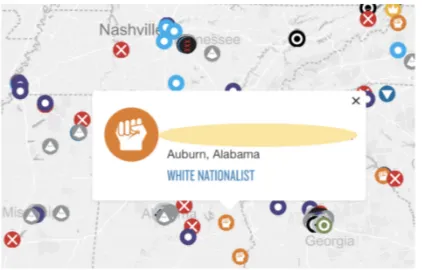
Figure 1: A portion of the hate group map published by the Southern Poverty Law Center (SPLC). Each marker represents a hate group. The markers with the same pattern indicate the corresponding hate groups share the same ideology. The white box shows an example of a hate group in Auburn, Alabama under the category of ”White Nationalist”. Due to the sensitivity of the data, we mask the name of the group.
classifications with only a small set of categories. To the best of our knowledge, the existing work on hate speech detection formulates the task as a classification problem with no more than seven classes. Building a model for more fine-grained multiclass classification is more challenging since it requires the model to capture finer distinctions between each class.
Moreover, fine-grained classification is neces-sary for fine-grained hate speech analysis. Fig-ure1is a portion of the hate group map published by the Southern Poverty Law Center (SPLC)2, where a hate group is defined as “an organization that based on its official statements or principles, the statements of its leaders, or its activities has beliefs or practices that attack or malign an en-tire class of people, typically for their immutable characteristics.” The SPLC divides the 954 hate groups in the United States into 17 categories
cording to their ideologies (e.g. Racist Skinhead, Anti-Immigrant, and others). The SPLC monitors hate groups throughout the United States by a va-riety of methodologies to determine the activities of groups and individuals: reviewing hate group publications and reports by citizens, law enforce-ment, field sources and the news media, and con-ducting their own investigations. Therefore, build-ing automatic classification models to differentiate between the social media posts from different hate groups is both challenging and of practical signif-icance.
In this paper, we propose a fine-grained hate speech classification task that separates tweets posted by 40 hate groups of 13 different hate group categories. Although CVAE is commonly used as a generative model, we find it can achieve compet-itive results and tends to be more robust when the size of the training dataset decreases, compared to the commonly used discriminative neural network models. Based on this insight, we design a Hierar-chical CVAE model (HCVAE) for this task, which leverages the additional hate group category (ide-ology) information for training. Our contributions are three-fold:
• This is the first paper on fine-grained hate speech classification that attributes hate groups to individual tweets.
• We propose a novel Hierarchical CVAE model for fine-grained tweet hate speech classification.
• Our proposed model improves the Micro-F1 score of up to 10% over the baselines.
In the next section, we outline the related work on hate speech detection, fine-grained text classifica-tion, and Variational Autoencoder. In Section 3, we explore the CVAE as a discriminative model, and our proposed method is described in Section4. Experimental results are presented and discussed in Section5. Finally, we conclude in Section6.
2 Related Work
2.1 Hate Speech Detection
An extensive body of work has been dedicated to automatic hate speech detection. Most of the work focuses on binary classification. Warner and Hirschberg(2012) differentiate between anti-semitic or not. Gao et al. (2017), Zhong et al.
(2016), andNobata et al. (2016) differentiate be-tween abusive or not. Waseem and Hovy(2016),
Burnap and Williams(2016), andDavidson et al.
(2017) focus on three-way classification.Waseem and Hovy (2016) classify each input tweet as racist hate speech, sexist hate speech, or neither.
Burnap and Williams (2016) build classifiers for hate speech based on race, sexual orientation or disability, while Davidson et al. (2017) train a model to differentiate among three classes: con-taining hate speech, only offensive language, or neither.Badjatiya et al.(2017) use the dataset pro-vided by Waseem and Hovy (2016) to do three-way classification. Our work is most closely re-lated to (Van Hee et al., 2015), which focuses on fine-grained cyberbullying classification. How-ever, this study only focuses on seven categories of cyberbullying while our dataset consists of 40 classes. Therefore, our classification task is much more fine-grained and challenging.
2.2 Fine-grained Text Classification
Our work is also related to text classification. Con-volutional Neural Networks (CNN) have been suc-cessfully applied to the text classification task.
Kim(2014) applies CNN at the word level while
Zhang et al. (2015) apply CNN at the character level. Johnson and Zhang(2015) exploit the word order of text data with CNN for accurate text cat-egorization. Socher et al. (2013) introduces the Recursive Neural Tensor Network for text classi-fication. Recurrent Neural Networks (RNN) are also commonly used for text classification (Tai et al., 2015; Yogatama et al., 2017). Lai et al.
(2015) and Zhou et al. (2015) further combine RNN with CNN.Tang et al.(2015) andYang et al.
(2016) exploit the hierarchical structure for doc-ument classification. Tang et al. (2015) generate from the sentence representation to the document representation while Yang et al. (2016) generate from the word-level attention to the sentence-level attention. However, the division of the hierarchies in our HCVAE is according to semantic levels, rather than according to document compositions. We generate from the category-level representa-tions to the group-level representarepresenta-tions. Moreover, the most commonly used datasets by these works (Yelp reviews, Yahoo answers, AGNews, IMDB reviews (Diao et al.,2014)) have no more than 10 classes.
2.3 Variational Autoencoder
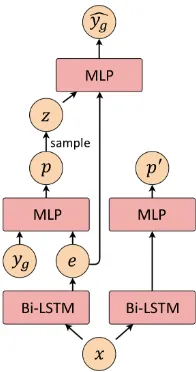
Figure 2: The structure of the baseline CVAE model during training. Bi-LSTM is a bidirectional LSTM layer. MLP is a Multilayer Perceptron.xis the embed-ded input text. ygis the ground truth hate group label.
ˆ
yg is the output prediction of the hate group. pis the posterior distribution of the latent variable zwhile p0 is the prior distribution ofz. Note that this structure is used for training. During testing, the posterior network is replaced by the prior network to computeyˆgand thus ygis not available during testing. Refer to Section3for detailed explanation.
many complicated generation tasks, such as hand-written digits (Kingma and Welling, 2013; Sali-mans et al., 2015), faces (Kingma and Welling,
2013;Rezende et al.,2014), and machine transla-tion (Zhang et al., 2016). CVAE (Larsen et al.,
2016; Sohn et al., 2015) is an extension of the original VAE framework that incorporates condi-tions during generation. In addition to image gen-eration, CVAE has also been successfully applied to several NLP tasks, such as dialog generation (Zhao et al., 2017). Although so far CVAE has always been used as a generative model, we ex-plore the performance of the CVAE as a discrim-inative model and further propose a hierarchical CVAE model, which exploits the hate group cate-gory (ideology) information for training.
3 CVAE Baseline
We formulate our classification task as the follow-ing equation:
Obj= X
(x,yg)∈X
logp(yg|x) (1)
wherex,ygare the tweet text and hate group label
respectively, X is the dataset. Instead of directly
parameterizingp(yg|x), it can be further written as
the following equation:
p(yg|x) =
Z
z
p(yg|z, x)p(z|x)dz (2)
wherezis the latent variable. Since the integration overz is intractable, we instead try to maximize the corresponding evidence lower bound (ELBO):
ELBO=E[logp(yg|z, x)]−
DKL[q(z|x, yg)||p(z|x)]
(3)
where DKL is the KullbackLeibler (KL)
diver-gence. p(yg|z, x) is the likelihood distribution,
q(z|x, yg)is the posterior distribution, andp(z|x)
is the prior distribution. These three distributions are parameterized bypϕ(yg|z, x),qα(z|x, yg), and
pβ(z|x). Therefore, the training loss function is:
L=LREC+LKL
=Ez∼pα(z|x,yg)[−logpϕ(yg|z, x)]+
DKL[qα(z|x, yg)||pβ(z|x)]
(4)
The above loss function consists of two parts. The first part LREC is the reconstruction loss.
Opti-mizing LREC can push the predictions made by
the posterior network and the likelihood network closer to the ground truth labels. The second part LKLis the KL divergence loss. Optimizing it can
push the output distribution of the prior network and that of the posterior network closer to each other, such that during testing, when the ground truth labelygis no longer available, the prior
net-work can still output a reasonable probability dis-tribution overz.
Figure 2 illustrates the structure of the CVAE model during training (the structure used for testing is different). The likelihood network pϕ(yg|z, x)is a Multilayer Perceptron (MLP). The
structure of both the posterior networkqα(z|x, yg)
and the prior network pβ(z|x) is a bidirectional
p). Thus during testing, the ground truth labels will not be used to make predictions.
We assume the latent variable z has a multi-variate Gaussian distribution: p = N(µ,Σ) for the posterior network, andp0 =N(µ0,Σ0)for the prior network. The detailed computation process is as follows:
e=f(x) (5)
µ,Σ =s(yg⊕e) (6)
µ0,Σ0=s0(f0(x)) (7)
wheref is the Bi-LSTM function andeis the out-put of the Bi-LSTM layer at the last time step. s is the function of the MLP in the posterior net-work and s0 is that of the MLP in the prior net-work. The notation⊕means concatenation. The latent variables z and z0 are randomly sampled fromN(µ,Σ) andN(µ0,Σ0), respectively. Dur-ing trainDur-ing, the input for the likelihood network isz:
ˆ
yg=w(z) (8)
wherewis the function of the MLP in the likeli-hood network. During testing, the prior network will substitute for the posterior network. Thus for testing, the input for the likelihood isz0instead of z:
ˆ
yg =w(z0) (9)
4 Our Approach
One problem with the above CVAE method is that it utilizes the group label for training, but ignores the available hate group category (ideology) infor-mation of the hate speech. As mentioned in Sec-tion 1, hate groups can be divided into different categories in terms of ideologies. Each hate group belongs to a specific hate group category. Con-sidering this hierarchical structure, the hate cate-gory information can potentially help the model to better capture the subtle differences between the hate speech from different hate groups. Therefore, we extend the baseline CVAE model to incorpo-rate the category information. In this case, the ob-jective function is as follows:
Obj= X
(x,yc,yg)∈X
logp(yc, yg|x)
= X
(x,yc,yg)∈X
logp(yc|x)+logp(yg|x, yc)
(10)
whereycis the hate group category label and
p(yc|x) =
Z
zc
p(yc|zc, x)p(zc|x)dzc (11)
p(yg|x, yc) =
Z
zg
p(yg|zg,x,yc)p(zg|x,yc)dzg (12)
where zc and zg are latent variables. Therefore,
the ELBO of our method is the sum of the ELBOs oflogp(yc|x)andlogp(yg|x, yc):
ELBO=E[logp(yc|zc, x)]−
DKL[q(zc|x, yc)||p(zc|x)]+
E[logp(yg|zg, x, yc)]−
DKL[q(zg|x, yc, yg)||p(zg|x, yc)]
(13)
During testing, the prior networks will substi-tute the posterior networks and the ground truth labels yc and yg are not utilized. Hence the
priorp(zg|x, yc) in the above equation cannot be
parametrized as a network that directly takes the ground truth labelycandxas inputs. Instead, we
parameterize it as shown in the right part of Fig-ure3. We assume thatu0 is trained to be a latent representation ofyc, so we useu0 andxas inputs
for this prior network.
According to the ELBO above, the correspond-ing loss functionLis the combination of the loss function for the category classification (Lc) and that for the group classification (Lg).
L=Lc+Lg, where
Lc=Ezc∼qα(zc|x,yc)[−logpϕ(yc|zc, x)]+
DKL[qα(zc|x, yc)||pβ(zc|x)], and
Lg =Ezg∼qη(zg|x,yc,yg)[−logpθ(yg|zg, x, yc)]+
DKL[qη(zg|x, yc, yg)||pγ(zg|x, u)]
(14)
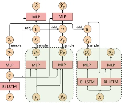
Figure 3 shows the structure of our model for training. By assuming the latent variableszc and
zg have multivariate Gaussian distributions, the
actual outputs of the posterior and prior networks are the mean and variance: pc = N(µc,Σc),
pg = N(µg,Σg) for the two posterior networks,
andp0c=N(µ0c,Σ0c),p0g =N(µ0g,Σ0g)for the two prior networks. Note that in addition to these four distributions, there is another distribution px = N(µx, σx) as shown in Figure 3. This
Figure 3: The structure of the HCVAE during train-ing. Bi-LSTM is a bidirectional LSTM layer. MLP is a Multilayer Perceptron. xis the embedded input text. yc andyg are the ground truth hate category label and hate group label. yˆc andyˆgare the output predictions of the hate category and hate group. zc,zg, andzc0 are latent variables. In the left dotted box are two poste-rior networks. In the right dotted box are two pposte-rior networks. Note that this structure is used for training. During testing, the posterior networks will be substi-tuted by the posterior networks (i.e. the left dotted box will be substituted with the right one) to computeyˆc andyˆg. Thusycandygare not available during testing. Refer to Section4for detailed explanation.
of the prior distribution) for both two posterior net-works and two prior netnet-works. With this basic dis-tribution, the two posterior networks only need to capture the additional signals learned fromx and labels. Similarly, the prior networks only need to learn the additional signals learned by the poste-rior networks. The detailed computation process during training is shown as the following equa-tions:
e=f(x) (15)
µx,Σx=sx(e) (16)
µc,Σc=sc(yc⊕e) (17)
µg,Σg=sg(yc⊕yg⊕e) (18)
µ0c,Σ0c=s0c(fc0(x)) (19)
wheref is the Bi-LSTM function and e is the out-put of the Bi-LSTM layer at the last time step.sx,
sc, sg, and s0c are the functions of four different
MLPs. fc0 is the Bi-LSTM function in the prior networkpβ(zc|x). The latent variableszx,zc,zg,
andzc0 are randomly sampled from the Gaussian distributionsN(µx,Σx), N(µc,Σc), N(µg,Σg),
andN(µ0c,Σ0c)respectively. As mentioned above,
Algorithm 1Train & Test Algorithm 1: functionTRAIN(X)
2: randomly initialize network parameters; 3: forepoch= 1, Edo
4: for(text, category, group)inXdo
5: get embeddingsxand one-hot vectorsyc,yg;
6: computeewith the Bi-LSTM; 7: computeµx,Σx,µc,Σc,µg,Σg;
8: samplezx=reparameterize(µx,Σx);
9: samplezc=reparameterize(µc,Σc);
10: samplezg =reparameterize(µg,Σg);
11: u=zx+zc;
12: v=u+zg;
13: computeyˆcandyˆgaccording to Eq.24-25;
14: LREC=BCE( ˆyc, yc) +BCE( ˆyg, yg);
15: computeµ0c,Σ0c;
16: samplezc0 =reparameterize(µ0c,Σ0c);
17: u0=zx+z0c;
18: computeµ0g,Σ0g;
19: LKL=DKL(pc||pc0) +DKL(pg||p0g);
20: L=LKL+LREC;
21: update network parameters onL; 22: end for
23: end for
24: end function
25:
26: functionTEST(X) 27: fortextinXdo
28: get embeddingsx;
29: computeewith the Bi-LSTM; 30: computeµx,Σx,µ0c,Σ
0
c;
31: samplezx=reparameterize(µx,Σx);
32: samplezc0 =reparameterize(µ0c,Σ0c);
33: u0=zx+zc0;
34: computeµ0g,Σ0g;
35: samplezg0 =reparameterize(µ0g,Σ0g);
36: v0=u0+zg0;
37: computeyˆcandyˆgaccording to Eq.26-28;
38: end for
39: end function
px is the basic distribution while pc, pg, p0c, and
p0g are trained to capture the additional signals. Therefore, zx is added to zc andzc0, then the
re-sultsu andu0 are further added tozg andzg0,
re-spectively, as shown in the following equations:
u0 =zx+zc0 (20)
µ0g,Σ0g =s0g(u0⊕fg0(x)) (21)
u=zx+zc (22)
v=u+zg (23)
where fg0 is the Bi-LSTM function and s0g is the function of the MLP in the prior network pγ(zg|x, u). +is element-wise addition. During
training, u and v are fed into the likelihood net-works:
ˆ
yc=wc(e⊕u) (24)
ˆ
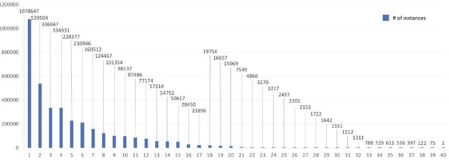
Figure 4: The distribution of the data for 40 hate groups. The X-Axis is each hate group. The Y-Axis is the number of tweets collected for each hate group.
wherewcandwgare the functions of the MLPs in
two likelihood networks. During testing, the prior networks will substitute the posterior networks, so the latent variable zg0 is randomly sampled from the Gaussian distributionsN(µ0g,Σ0g), and the last four equations above (Equation 22 - 25) will be replaced by the following ones:
ˆ
yc=wc(e⊕u0) (26)
v0 =u0+zg0 (27)
ˆ
yg =wg(e⊕v0) (28)
Algorithm 1illustrates the complete training and testing process. BCE refers to the Binary Cross Entropy loss. Note that during training, the ground truth category labels and group labels are fed to the posterior network to generate latent variables. But during testing, the latent variables are generated by the prior network, which only utilizes the texts as inputs.
5 Experiments
5.1 Dataset
We collect the data from 40 hate group Twit-ter accounts of 13 different hate ideologies, e.g., white nationalist, anti-immigrant, racist skinhead, among others. The detailed themes and core val-ues behind each hate ideology are discussed in the SPLC ideology section.3 For each hate ide-ology, we collect a set of Twitter handles based on hate groups identified by the SPLC center.4 For
3
https://www.splcenter.org/fighting-hate/extremist-files/ideology
4 https://www.splcenter.org/fighting-hate/extremist-files/groups
each hate ideology, we select the top three han-dles in terms of the number of followers. Due to ties, there are four different groups in several categories of our dataset. The dataset consists of all the content (tweets, retweets, and replies) posted with each account from the group’s incep-tion date, as early as 07-2009, until 10-2017. Each instance in the dataset is a tuple of (tweet text, hate category label, hate group label). The com-plete dataset consists of approximately 3.5 million tweets. Note that due to the sensitive nature of the data, we anonymously reference the Twitter han-dles for each hate group by using IDs throughout this paper. The distribution of the data is illus-trated in Figure4.
5.2 Experimental Settings
In addition to the discriminative CVAE model de-scribed in Section3, we implement for other base-line methods and an upper bound model as fol-lows.
Support Vector Machine (SVM): We implement an SVM model with linear kernels. We use L2 reg-ularization and the coefficient is 1. The input fea-tures are the Term Frequency Inverse Document Frequency (TF-IDF) values of up to 2-grams.
Logistic Regression (LR): We implement the Lo-gistic Regression model with L2 regularization. The penalty parameter C is set to 1. Similar to the SVM model, we use TF-IDF values of up to 2-grams as features.
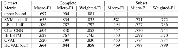
Dataset Complete Subset
Metric Macro-F1 Micro-F1 Weighted-F1 Macro-F1 Micro-F1 Weighted-F1
upper bound .697 .904 .881 – – –
SVM + tf-idf .653 .834 .835 .521 .771 .772
LR + tf-idf .586 .787 .792 .494 .727 .736
Char-CNN .604 .840 .853 .457 .730 .744
Bi-LSTM .627 .767 .745 .353 .599 .570
CVAE .520 .799 .830 .453 .774 .784
[image:7.595.111.483.61.162.2]HCVAE (our) .664 .844 .858 .469 .787 .799
Table 1: Experimental results. Complete: The performance achieved when 90% of the entire dataset is used for training. Subset: The performance achieved when only 10% of the dataset is used for training. The best results are in bold.
The configurations of the convolutional layers are kept the same as those in (Zhang et al.,2015).
Bi-LSTM: The model consists of a bidirectional LSTM layer followed by a linear layer. The em-bedded tweet textxis fed into the LSTM layer and the output at the last time step is then fed into the linear layer to predictyˆg.
Upper Bound: The upper bound model also con-sists of a bidirectional LSTM layer followed by a linear layer. The difference between this model and Bi-LSTM is that it takes the tweet textxalong with the ground truth category label yc as input
during both training and testing. The LSTM layer is used to encode x. The encoding result is con-catenated with the ground truth category label and then fed into the linear layer to give the prediction of the hate groupyˆg. Since it utilizesycfor
predic-tion during testing, this model sets an upper bound performance for our method.
For the baseline CVAE, Bi-LSTM, the upper bound model, and the HCVAE, we use randomly initialized word embeddings with size 200. All the neural network models are optimized by the Adam optimizer with learning rate 1e-4. The batch size is 20. The hidden size of all the LSTM layers in these models is 64 and all the MLPs are three-layered with non-linear activation function Tanh. For the CVAE and the HCVAE, the size of the la-tent variables is set to 256.
All the baseline models and our model are eval-uated on two datasets. We first use the complete dataset for training and testing. 90% of the in-stances are used for training and the rest for test-ing. In order to evaluate the robustness of the baline models and our model, we also randomly se-lected a subset (10%) of the original dataset for training while the testing dataset is fixed. Since the upper bound model is used to set an upper bound on performance, we do not evaluate it on
the smaller training dataset. We use Macro-F1, Micro-F1, and Weighted-F1 to evaluate the classi-fication results. As shown in Figure4, the dataset is highly imbalanced, which causes problems for training the above models. In order to alleviate this problem, we use a weighted random sampler to sample instances from the training data. How-ever, the testing dataset is not sampled, so the dis-tribution of the testing dataset remains the same as that of the original dataset. This allows us to eval-uate the models’ performance on the data with a realistic distribution.
5.3 Experimental Results
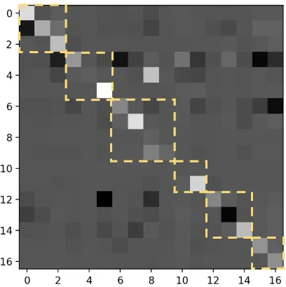
Figure 5: This figure compares a subset (17 hate groups of 6 categories) of the predictions made by the baseline CVAE and the HCVAE. The X and Y axes are the in-dex of each hate group. The hate groups of the same category are grouped together as shown in the dashed squares. The color of the grid(i, j)is mapped from rhcvae(i, j)−rcvae(i, j), wherer(i, j)is the fraction of the groupi’s instances among the instances predicted as the groupj. A higher difference value corresponds to a lighter color. A grid darker than the background is mapped from a negative value while a grid lighter than the background is mapped from a positive one.
variable while the CVAE model explicitly mod-els the posterior and likelihood distributions over the latent variable. The result is that, during test-ing, the inference strategy of the Bi-LSTM model and the Char-CNN model is actually comparing the compressed text to the compressed instances in the training dataset while the strategy of the CVAE-based models is to compare the prior dis-tributions over the latent variable. Compared with the compressed text, prior distributions may cap-ture higher level semantic information and thus enable better generalization.
By further utilizing the hate category label for training, the HCVAE outperforms the baseline CVAE on all three metrics. Figure 5 illustrates the difference between the predictions made by the HCVAE and the CVAE. As shown in the fig-ure, most of the lighter girds are in the dashed squares while most of the darker girds are out-side. This indicates that the HCVAE model tends to correct the prediction of the CVAE’s misclas-sified instances to be closer to the ground truth. In most cases, the misclassified instances can be directly corrected to the ground truth (the
diago-Figure 6: The F1 score achieved by our method on each hate group. The Y-axis is the F1 score. The X-axis is the hate group sorted by the number of instances in the dataset from larger to smaller. The dashed line shows the F1 scores and the solid line is the corresponding trendline.
nal). In other cases, they are not corrected to the ground truth but are corrected to the hate groups of the same categories as the ground truth (the dashed squares). This shows that additional ideology in-formation is useful for the model to better capture the subtle differences among tweets posted by dif-ferent hate groups.
Although our method outperforms the baseline methods, there is still a gap between its perfor-mance and the upper bound perforperfor-mance. We an-alyze this in the following section.
5.4 Error Analysis
[image:8.595.309.532.63.192.2]into the instances in the testing dataset, the perfor-mance can be less satisfactory. This is a common problem for all the methods, which is the cause of the significantly lower Macro-F1 scores.
Another type of error is caused by the noisy dataset. Take, for instance, the tweet fromGroup3 under the category “ku klux klan”:we must secure the existence of our people and future for the White Children !!Our model classifies it as fromGroup4 under the category “neo nazi”, which makes sense but is an error.
6 Conclusion
In this paper, we explore the CVAE as a discrimi-native model and find that it can achieve compet-itive results. In addition, the performance of the CVAE-based models tend to be more stable than that of the others when the dataset gets smaller. We further propose an extension of the basic dis-criminative CVAE model to incorporate the hate group category (ideology) information for train-ing. Our proposed model has a hierarchical struc-ture that mirrors the hierarchical strucstruc-ture of the hate groups and the ideologies. We apply the HC-VAE to the task of fine-grained hate speech clas-sification, but this Hierarchical CVAE framework can be easily applied to other tasks where the hier-archical structure of the data can be utilized.
References
Pinkesh Badjatiya, Shashank Gupta, Manish Gupta, and Vasudeva Varma. 2017. Deep learning for hate speech detection in tweets. In Proceedings of the 26th International Conference on World Wide Web Companion, pages 759–760. International World Wide Web Conferences Steering Committee.
Pete Burnap and Matthew L Williams. 2016. Us and Them: Identifying Cyber Hate on Twitter across Multiple Protected Characteristics. EPJ Data Sci-ence, 5(1):11.
Thomas Davidson, Dana Warmsley, Michael Macy, and Ingmar Weber. 2017. Automated hate speech detection and the problem of offensive language. arXiv preprint arXiv:1703.04009.
Qiming Diao, Minghui Qiu, Chao-Yuan Wu, Alexan-der J Smola, Jing Jiang, and Chong Wang. 2014. Jointly modeling aspects, ratings and sentiments for movie recommendation (jmars). InProceedings of the 20th ACM SIGKDD international conference on Knowledge discovery and data mining, pages 193– 202. ACM.
Lei Gao, Alexis Kuppersmith, and Ruihong Huang. 2017. Recognizing explicit and implicit hate speech using a weakly supervised two-path bootstrapping approach. In Proceedings of the Eighth Interna-tional Joint Conference on Natural Language Pro-cessing (Volume 1: Long Papers), volume 1, pages 774–782.
Sepp Hochreiter and J¨urgen Schmidhuber. 1997. Long short-term memory. Neural computation, 9(8):1735–1780.
Rie Johnson and Tong Zhang. 2015. Effective use of word order for text categorization with convolu-tional neural networks. InProceedings of the 2015 Conference of the North American Chapter of the Association for Computational Linguistics: Human Language Technologies, pages 103–112.
Yoon Kim. 2014. Convolutional neural networks for sentence classification. InProceedings of the 2014 Conference on Empirical Methods in Natural Lan-guage Processing (EMNLP), pages 1746–1751.
Diederik P Kingma and Max Welling. 2013. Auto-encoding variational bayes. arXiv preprint arXiv:1312.6114.
Siwei Lai, Liheng Xu, Kang Liu, and Jun Zhao. 2015. Recurrent convolutional neural networks for text classification. In AAAI, volume 333, pages 2267– 2273.
Anders Boesen Lindbo Larsen, Søren Kaae Sønderby, Hugo Larochelle, and Ole Winther. 2016. Autoen-coding beyond pixels using a learned similarity met-ric. InProceedings of the 33rd International Con-ference on International ConCon-ference on Machine Learning-Volume 48, pages 1558–1566. JMLR. org.
Chikashi Nobata, Joel Tetreault, Achint Thomas, Yashar Mehdad, and Yi Chang. 2016. Abusive lan-guage detection in online user content. In Proceed-ings of the 25th international conference on world wide web, pages 145–153. International World Wide Web Conferences Steering Committee.
Danilo Jimenez Rezende, Shakir Mohamed, and Daan Wierstra. 2014. Stochastic backpropagation and approximate inference in deep generative models. In International Conference on Machine Learning, pages 1278–1286.
Tim Salimans, Diederik Kingma, and Max Welling. 2015. Markov chain monte carlo and variational in-ference: Bridging the gap. InInternational Confer-ence on Machine Learning.
Kihyuk Sohn, Honglak Lee, and Xinchen Yan. 2015. Learning structured output representation using deep conditional generative models. InAdvances in Neural Information Processing Systems.
Kai Sheng Tai, Richard Socher, and Christopher D Manning. 2015. Improved semantic representations from tree-structured long short-term memory net-works. In Proceedings of the 53rd Annual Meet-ing of the Association for Computational LMeet-inguistics and the 7th International Joint Conference on Natu-ral Language Processing (Volume 1: Long Papers), volume 1, pages 1556–1566.
Duyu Tang, Bing Qin, and Ting Liu. 2015. Docu-ment modeling with gated recurrent neural network for sentiment classification. In Proceedings of the 2015 conference on empirical methods in natural language processing, pages 1422–1432.
Cynthia Van Hee, Els Lefever, Ben Verhoeven, Julie Mennes, Bart Desmet, Guy De Pauw, Walter Daele-mans, and V´eronique Hoste. 2015. Detection and Fine-grained Classification of Cyberbullying Events. In RANLP’15: International Conference Recent Advances in Natural Language Processing, pages 672–680.
William Warner and Julia Hirschberg. 2012. Detecting Hate Speech on the World Wide Web. InACL’12: Proceedings of the 2nd Workshop on Language in Social Media, pages 19–26. Association for Com-putational Linguistics.
Zeerak Waseem and Dirk Hovy. 2016. Hateful sym-bols or hateful people? predictive features for hate speech detection on twitter. In Proceedings of the NAACL student research workshop, pages 88–93.
Zichao Yang, Diyi Yang, Chris Dyer, Xiaodong He, Alex Smola, and Eduard Hovy. 2016. Hierarchi-cal attention networks for document classification. InProceedings of the 2016 Conference of the North American Chapter of the Association for Computa-tional Linguistics: Human Language Technologies, pages 1480–1489.
Dani Yogatama, Chris Dyer, Wang Ling, and Phil Blun-som. 2017. Generative and discriminative text clas-sification with recurrent neural networks. arXiv preprint arXiv:1703.01898.
Biao Zhang, Deyi Xiong, Hong Duan, Min Zhang, et al. 2016. Variational neural machine translation. In Proceedings of the 2016 Conference on Empiri-cal Methods in Natural Language Processing, pages 521–530.
Xiang Zhang, Junbo Zhao, and Yann LeCun. 2015. Character-level convolutional networks for text clas-sification. In Advances in neural information pro-cessing systems, pages 649–657.
Tiancheng Zhao, Ran Zhao, and Maxine Eskenazi. 2017. Learning discourse-level diversity for neural
dialog models using conditional variational autoen-coders. In Proceedings of the 55th Annual Meet-ing of the Association for Computational LMeet-inguistics (Volume 1: Long Papers), volume 1, pages 654–664.
Haoti Zhong, Hao Li, Anna Cinzia Squiccia-rini, Sarah Michele Rajtmajer, Christopher Grif-fin, David J Miller, and Cornelia Caragea. 2016. Content-Driven Detection of Cyberbullying on the Instagram Social Network. In IJCAI’16: Proceed-ings of the 25th International Joint Conference on Artificial Intelligence, pages 3952–3958.