A Nonlinear C-UPFC Control Design for Power Transmission Line Applications

A Nonlinear C-UPFC Control Design for Power

Transmission Line Applications

H.Ghane , S.K.Y.Nikravesh

Abstract— The C-UPFC is an elegant FACTS device and consists of three voltage source inverters (VSI) with common DC link. One of the converters is connected in parallel at the midpoint of line and the other two converters are connected in series. This paper deals with design and evaluation of a novel nonlinear control scheme based on input output feedback linearization technique for improving power transmission line dynamics. The simulation results indicate that with proposed nonlinear control, the C-UPFC is capable of independently controlling the active and reactive power flows at the both ends of line and the magnitude of AC voltage at line mid point. Simultaneously keep the DC link voltage at constant value.

Index Terms— FACTS, Nonlinear Control, C-UPFC,

Feedback Linearization

I. INTRODUCTION

The increasing demand for electric power requires to increase the transmission capabilities. Under de-regulation, however, electric utilities are reluctant to build new transmission line for economic and environmental consideration. The system is operated in ways, which lead to maximum use of existing transmission facilities, and this is not achievable unless new devices are installed on the transmission line to ensure proper performance of power system [1-3]. In recent years, the advances in power electronics have led to the development of the Flexible AC transmission system (FACTS). FACTS is designed to enhance power system capability and its dynamic by using reliable and high speed electronic devices. In these devices, with the help of high power GTO devices, the cumbersome rotating synchronous condenser can be replaced by the solid-state synchronous voltage source (SVS) in power transmission applications. The SVS is similar to an ideal synchronous machine in which a balanced three-phase sinusoidal voltage, with controllable magnitude and phase angle, is generated at the desired fundamental frequency. When connected in shunt or in series with a transmission line, the SVS can internally generate inductive and capacitive reactive power. It can also generate or absorb real power if a real power source is connected at the dc-link.[4]-[5].

Manuscript received December 4, 2008.

Both authors are with the Electrical Engineering Department, Aboureyhan Building, Amirkabir University of Technology (Tehran Polytechnic). Tehran, Iran

H. Ghane (corresponding author to provide phone: +982164543398; fax: +982166406469; e-mail: [email protected], also Hghane@ aut.ac.ir).

S.K.Y.Nikravesh,.(phone:+98216466009;[email protected]).

The UPFC is the most elegant device of FACTS controllers. Two back-to-back connected SVS systems with one SVS connected in shunt and the other in series with the transmission line produces what is known as a

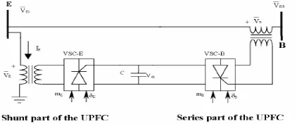
unified power flow controller (UPFC).The power circuit of a UPFC, (see Fig.1), is composed of an excitation transformer (ET), a boosting transformer (BT), Two three phase GTO based voltage source converters (VSC), and a DC link capacitor. It is clear that m_E,m_B,δ δ_E, _B (the amplitude modulation ratios and phase angles of corresponding sources) act as the input control signals for UPFC [6]-[10].

In this topology, by using mentioned four control variables, it is possible to control the line active power flow, sending or receiving end reactive power and shunt converter AC bus voltage. Because of the limited number of control variables, the ordinary UPFC is not capable of controlling more than four variables in power transmission system, simultaneously. To overcome this problem, a new topology of UPFC has been developed in [11] and [12]. This new FACTS device is named center node UPFC (C-UPFC) installed at the midpoint of transmission line as shown in Fig. 2.

[image:1.595.329.540.661.749.2]

Since C-UPFC is a new developed configuration of UPFC, the researches and control schemes designed for it are limited. It was first introduced in [11], with tow separate DC links, (one for shunt VSC and one for tow series VSCs), after that, [12] improve its configuration with using one DC link for all three VSCs. But just linear PI controllers are investigated and its scope is limited to steady state analysis. The last published paper about C-UPFC performance is [13] which investigate C-UPFC's transient model in transmission line and like previous papers linear control is applied in it. In this paper after state space modeling of C-UPFC in transmission line, nonlinear controller based on input-output feedback linearization, will be designed to ensure that under all operating conditions the performance of our controller is guaranteed. Indeed the superior capabilities of this device will be discussed. It will be shown that this device can control the active and reactive powers of sending and receiving ends and simultaneously can regulate the midpoint voltage magnitude and DC link voltage.

[image:2.595.73.274.51.146.2]

Fig. 2. General configuration of C-UPFC

At the first the dynamic equations of transmission system including the C-UPFC will be derived and state space modeling will be presented. Section two consists of some manipulations on state space equations. Then outputs of interest described in terms of state variables. At the next section the input-output feedback linearization technique will be briefly described and then applied on the proposed system. This section is followed by the proof of exponential convergence of outputs to their reference values. And finally in the last section, results of simulations will be compared with existing published researches and advantages of presented nonlinear MIMO controller over so far used controllers for C-UPFC will be clarified.

II. SYSTEM DYNAMIC

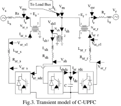
Fig.3 shows the transient model of C-UPFC in transmission line [13]. In which, theLsh, Lsr s_ ,Lsr r_ and

sh

R , R_{sr s_} , R_{sr r_} represent leakage inductances of

transformers and losses of inverters and transformers. By writing Kirchhoff's Voltage Law for three converters and transformation of resulting equations into d-q frame, three pair of differential equations are obtained which can be used as part of state space modeling as below;

_

_ _ _ _ _ _

_

_ _ _ _ _ _

_

_

_ _ _ _ _ _

_ _ sr sd

sr s sd sr s sr sd sr sd sr s sr sd sr s

sr s sq sr s sr sq sr sq sr s sr sq sr sq

sr rd

sr r rd sr r sr rd sr rd sr r sr rq sr r

s sr rq d

I

N E R I V L I

dt L

d N E R I V L I

I dt

d I

N E R I V L I

dt L

d N

I dt

ω ω

ω

− − − +

=

− − − −

− − − +

= −

⎡ ⎤

⎢ ⎥ ⎡ ⎤

⎥

⎢ ⎥ ⎢_{⎣ ⎦}

⎢ ⎥

⎣ ⎦

⎡ ⎤

⎢ ⎥

⎢ ⎥

⎢ ⎥

⎣ ⎦ r_r rq sr_r sr_rq sr_rq sr_r sr_rd E −R I −V −ωL I

⎡ ⎤

⎢ ⎥

⎣ ⎦

shd

sh md sh shd shd sh shq sh

sh rq sh shq shq sh shd shq

d I

N V R I V L I

dt L

d N E R I V L I

I dt

ω ω

− + + +

=

− − + −

⎡

⎤

⎢

⎥ ⎡

⎤

⎢

⎥ ⎢

_⎣

⎥

⎢

⎥

⎣

⎦

⎦

(1)

In which N_{sr s_} ,N_{sr r_} ,N_sh represent the transformer ratio of three VSCs. The output voltages of three VSCs are appeared in the above relations. Based on [14] with some modification, It is possible to describe the output voltage of

every VSC in terms of its control input as below

;

1

2 _{, _ , , _}

1

2

id i dc i

iq i dc i

V m V Cos

i sr s sh sr r

V m V Sin

δ

δ =

= =

⎧

⎪

⎨

⎪

⎩

(2)

Now the dynamic of DC link voltage must be calculated.

According to [14], its dynamic is obtained with some modification to include the third series converter. Anyway

after transforming into d-q frame, the DC link voltage dynamic is obtained as below [14];

3 1 ( ) 2 2

3 1 _{_}

( _{_} ) _{_ _} _ 2 2

3 1 _{_}

( _{_} ) _{_ _} _ 2 2

sh sh

Cos Sin

d _{I shd}

V_DC m_sh

I shq

dt C

I sr sd m_{sr s} Cos _{sr s} Sin _{sr s}

I sr sq C

I sr rd m_{sr r} Cos _{sr r} Sin _{sr r}

I sr rq C

δ δ

δ δ

δ δ

⎡ ⎤

⎣ ⎦

=

+

+

⎡

⎤

⎢

⎥

⎣

⎦

⎡

⎤

⎡

⎤

⎣

_{⎦ ⎢⎣}

_⎦

⎡

⎤

⎡

⎤

⎣

_{⎦ ⎢}

_⎣

_⎥

_⎦

⎥

(3)

[image:2.595.325.532.218.399.2]

As stated earlier, in the C-UPFC control scheme, ac-bus voltage V_m control is one of our final objectives.

Fig.3. Transient model of C-UPFC

It is noticeable that in the presented control strategy it is

assumed that is aligned with the axes of mentioned

d-q frame. In addition the variation of load current is supposed

to be negligible and voltage sources have constant values.

With this assumptions, the dynamic equation for is

obtained as follows with reference to Fig.3.

m

V

m

V

( ) (

m sd s shd rd ld s shq rq lq

V =V −R I +I +I −Lω I +I +I ) (4)

_ _

_ _

( )

( )

m s sh shd sr r sr rd

s sh shq sr r sr rq

d d

V R N I N I

dt dt

d d

L N I N I

dt dt

ω

= − +

− +

(5)

III. STATE SPACE MODELING

After rearrangement of equations (1), (3), and (5) and taking the ac currents of VCSs, DC link voltage, and ac bus voltage as state variables, the complete state space model is expressed as follows;

ˆ ( ) ( , )

x = F x +B x u (6)

In which;

_ _ _ _

_ _ _ _

ˆ

T shd shq sr sd sr sq sr sd sr rq dc m

T sh sh sr s sr s sr r sr r

x I I I I I I V V

u m δ m δ m δ

=

=

⎡ ⎤

⎣ ⎦

⎡ ⎤

⎣ ⎦

And;

By taking _i i

i N K

L

= and _Ti Ri

Li

1 2 8 1 2

_ _ _ 3 _ _ 4 _ 8 _ _ _

_ _ 3 _ _ _ 4 _ _ _ _ _ 1 [( ) ( ) ] (1 ) 1 [( ) ( ) ] (1 ) ( ) 1 [( (1 _r)

sh sh

sh

sr s sr s s sr s sr s sr s s sr s sr s sd sr s sr s s

sr s sr s s sr s sr s s sr s sr s sq sr s sr s s

sr sr r sr r

T x x K x

x T x

K N R T x K N L x K x K V

K N L

K N L x K N R T x K V

K N L

F x

K

K N L

ω ω ω ω ω ω − − + − − + − + − + − + − − + = + 1 2 3

_ _ _ 5 _ _ 6 _ 8 _

_ _ 5 _ _ _ 6 _ _ _

_ 3 _ 4

( ) ( ) ( ) ( ) ] 1 [( ) ( ) ] (1 ) 0 ( ) ( ) r

r sr r r sr r sr r sr r r sr r sr r rd

sr r sr r r sr r sr r r sr r sr r rq sr r sr r

s sr s s sr s

f x

f x

f

N R T x K N L x K x K V

K N L x K N R T x K V

K N L

R N f x L N f x

ω ω ω ω ω = − + − + − − + − − + − −

⎡

⎤

⎢

⎥

⎢

⎥

⎢

⎥

⎢

⎥

⎢

⎥

⎢

⎥

⎢

⎥

⎢

⎥

⎢

⎥

⎢

⎥

⎢

⎥

⎢

⎥

⎢

⎥

⎢

⎥

⎣

⎦

4 5 6 7 8 ) ( ) ( ) ( ) ( ) ( ) x f x f x f x f x f x ⎡ ⎤ ⎢ ⎥ ⎢ ⎥ ⎢ ⎥ ⎢ ⎥ ⎢ ⎥ ⎢ ⎥ ⎢ ⎥ ⎢ ⎥ ⎢ ⎥ ⎢ ⎥ ⎢ ⎥ ⎣ ⎦

the six objectives of proposed control scheme are specified. They include sending and receiving active and reactive It is obvious that the state space model is non-affine.

Because it is much more comfortable to deal with an affine model, with some modification on inputs the system can be presented in an affine model as follows;

power, midpoint ac voltage and DC link voltage. Thus output vector is established as follows;

1 5 _

2 6 _

_

_ _ _

sh sh sh sr r sr r sr r

sh sh sh sr r sr r sr r

u m K Cos u m K Cos

u m K Sin u m K Sin

δ δ

δ

= =

= =

[

]

T

s s r r m dc

y = P Q P Q V V (10)

δ

_ _ 3 _ _

4 _ _

sr s sr s sr s

sr s sr s sr s

u m K Cos

u m K Sin

δ δ

=

= (7)

In the following by writing outputs in terms of state variables, the state space modeling is completed.

_ 3 4 sr_s 4 3

_ 5 6 _ 6 5

8 7 3 ( ) 2 3 ( ) 2 3 ( ) ( ) 2 3 ( ) 2

sr s sd sq

sd sq

sr r rd rq

sr r rd rq

N V x V x

N V x V x

N V x V x

y h x

N V x V x

x x ⎡ ⎤ + ⎢ ⎥ ⎢ ⎥ ⎢ ₋ ⎥ ⎢ ⎥ ⎢ ⎥ ⎢ ₊ ⎥ = _{= ⎢ ⎥} ⎢ ⎥ ⎢ ₋ ⎥ ⎢ ⎥ ⎢ ⎥ ⎢ ⎥ ⎢ ⎥ ⎣ ⎦

Thus by using above transformation, the resulting affine model is as below;

( ) ( )

x=F x +B x u (8) ₍₁₁₎

In which B x( ) is a 8 matrix whose nonzero elements

are listed below;

6 × 11 22 7 33 44 7 55 66

71 72 2 3

74 75 5 76 6

83 7 ( ) ( ) ( ) ( ) (1 ) _ _ _ ( ) ( ) (1 ) _ _ _ 3 3

( ) ₁, ( ) , ( ) 73

2 2

3 3

( ) ₄ ( ) , ( )

2 2 _ ( ) (1 _ _ , x B x B x

Lsh

x B x B x

L_{sr s} K_{sr s}N_{sr s s}L

x B x B x

L_{sr r} K_{sr r}N_{sr r r}L

B x x B x x B x x

C C

B x x B x x B x x

C C

R N_{s sr s} B x

L_{sr s} K_{sr s}N

− = = − = = + − = = + = = = = = = = +

And hereby the complete state space model is ready to apply the proposed nonlinear control on it in the next section.

IV. NONLINEARCONTROLDESIGN

3 2 3 2 C C 7 ) _ x L sr s s

A. A brief review of feedback linearization Scheme

A brief review of nonlinear control using feedback

linearization is presented here. Without loss of generality,

the following MIMO (multi input and multi output) system is considered.

( ) ( ) ( )

x f x b x u

y h x

= + = (12) 84 7 _ ( ) (1 ) _ _ _

L N_{s sr s}

B x x

L_{sr s} K_{sr s}N_{sr s s}L

ω =

+

(9) _Where x is a n dimensional state vector,

represents the Control inputs, y stands for dimensional output vector,

( l)

u ∈\ l

fand are smooth vector fields, and is a

smooth scalar function. The input–output linearization of the above MIMO system is achieved by differentiating y of the

b h

l

system until the inputs appear explicitly. Thus, by differentiating Eq. (11),

1

( ) , 1, ...,

m

i f i bj i j j

y L h L h u i

=

∑

= + =

(13)

Where L h_f and L h_b

( )

represent the Lie derivatives of

with respect to

( ) h x f x ) ( ) i h x

and ; respectively. The key point is

that, if for all j; then the inputs do not

appear in (10) and further differentiation is to be repeated as

( )

b x

0 =

(r_i−1

bj f

L L

( ) ( ) ( 1) 1

( ) ,

l

r_i r_i r_i

i f i bj f i j

j

y L h L L − h u i

=

∑

= + =1, ...,l (14)

Such that for at least one j and in this step

is defined as relative degree of output. This

procedure is repeated for each output . Thus, there will be

a set of l equations given by

( 1)

0

r_i bj f i

L L − h ≠

ri ith i y 1 ( ) 1 1 ( ) ( ) ( ) l r r l l y u

L x M x

u y = +

⎡

⎤

⎡ ⎤

⎢

⎥

⎢ ⎥

⎢

⎥

_{⎢ ⎥}

⎣ ⎦

⎣

⎦

# # (15)

Where M x( ) and L x( ) are expressed by

1 1 1 1 1 1 1 1 1 1 ( ) l l l r r

b f b_l f

r r

b

b f l f l

L L h L L h

M x

L L h L L h

− − − − =

⎡

⎤

⎢

⎥

⎢

⎥

⎢

⎥

⎣

⎦

"

# " #

"

(16)

1

1( )

( ) ( ) l r f r f l

L h x

L x

L h x

⎡

⎤

⎢

⎥

= ⎢

⎢

⎥

⎣

⎦

#

⎥

(17)

( )

M x is called as the decoupling matrix for the MIMO

system. If M x( )is nonsingular, then the control can be

obtained as: u 1 1 1 1 ( ) ( ) ( ) l l u v

u M x L x M x

u v − − =

⎡ ⎤

⎢ ⎥

=− +

⎡ ⎤

⎢ ⎥

⎢ ⎥

⎢ ⎥

⎣ ⎦

⎣ ⎦

# #

]

# (18)

Where

[

is the new set of inputs defined by

the designer. The resultant dynamics of the system with new control is easily obtained by substitution of Eq. (18) into

1

T l

v " v

Eq. (15) and is given by

1

( ) 1 1

( )_l

r r l l y v v y =

⎡

⎤ ⎡ ⎤

⎢

⎥ ⎢ ⎥

⎢

⎥ ⎢ ⎥

_{⎣ ⎦}

⎣

⎦

# (19)

It is readily noticed that the input–output relation in Eq.(19) is decoupled and linear. Thus linear control scheme can be used to control the literalized system.

B. C-UPFC Nonlinear Control Design

For applying input output feedback linearization scheme on the resultant system in the section III, it is needed to differentiate from outputs as described above.

( ) ( )

y =L x +M x u (20)

In which L x( ) and M x( )are 6 1× and 6×6 matrixes which their elements are described as below;

The six elements of L x( ) are:

1 _ 3 4

2 _ 4

3 _ 5

4 _ 6

5 8 3 ( ) [ ( ) ( )] 2 3 ( ) [ ( ) ( )] 2 3 ( ) [ ( ) ( ) 2 3 ( ) [ ( ) ( )] 2 ( ) ( )

sr s sd sq

sr s sd sq

sr r rd rq

sr r rd rq

3

6

5

L x N V f x V f x

L x N V f x V f x

L x N V f x V f x

L x N V f x V f x

L x f x

= +

= −

= +

= −

=

6( ) 7( ) 0

L x = f x = (21)

And the nonzero elements of M x( ) are:

7 13 _ _ _ _ 7 14 _ _ _ _ 7 23 _ _ _ _ 7 23 _ _ _ _ 7 35 _ _ _ _ 3 ( )

2 (1 )

3 ( )

2 (1 )

3 ( )

2 (1 )

3 ( )

2 (1 )

3 ( )

2 (1

sd sr s

sr s sr s sr s s

sq sr s

sr s sr s sr s s

sq sr s

sr s sr s sr s s

sd sr s

sr s sr s sr s s

rd sr r

sr r sr r sr V x

M x N

L K N L

V x

M x N

L K N L

V x

M x N

L K N L

V x

M x N

L K N L

V x

M x N

L K N

= − + = − + = + = − + = − + 7 36 _ _ _ _ 7 45 _ _ _ _ 7 46 _ _ _ _

53 83 53 84

)

3 ( )

2 (1 )

3 ( )

2 (1 )

3 ( )

2 (1 )

( ) ( ) , ( ) ( )

r r

rq sr r

sr r sr r sr r r

rq sr r

sr r sr r sr r r

rd sr r

sr r sr r sr r r L

V x

M x N

L K N L

V x

M x N

L K N L

V x

M x N

L K N L

M x B x M x B x

= − + = + = − + = =

[

6 1 2 3 4 5 6

3 ( )

2

]

M x x x x x x x

C

= (22)

1

( )( ( ))

u=M− x v−L x (23)

By applying Eq.(23) in Eq.(20) the resultant linear relation between input and output vector is generated as follows;

y =v (24)

In whichv, is the new input vector and is determined such

that exponentially convergence of error signals to zero is guaranteed. To achieve this goal, is defined as v

( _ref ) _ref

v= y −y = +e y (25)

ref

e= y −y (26)

Substituting Eq.(25) and Eq.(25) in Eq.(24) lead to

0

e+ =e (27)

It is clear that the error signal, , is exponentially convergent to zero. Even it is possible to increase the convergence rate of error by some modification applied on

as bellow;

e

v

( _ref ) _ref

v= y −y =Ke+ y (28)

That leads to

0

e+Ke= (29)

In which K is a proportional matrix gain and is

determined by assigning desired poles on the left-half s-plane. Thus, asymptotic tracking control to the reference with the desired convergence rate can be achieved.

At the next section the simulation results are compared with just linear controller and the superior advantages of nonlinear control like as fast and exponentially convergence of outputs even in affront of fast changing reference values, are clarified.

V. SIMULATION RESULTS

The proposed nonlinear control scheme for C-UPFC is evaluated by computer simulation in MATLAB/SIMULINK. The values of parameters used in simulations are listed below, in the tables. In Table.1 the machine parameters including nominal voltage and power, impedance and phase are illustrated.

Table1. Machines Parameters Value

It is noticeable that in table.1, the line impedance is included in machine impedance in per unit.

In table.2, each VSC’s parameters consisting of leakage inductance, resistor and turn ratio of corresponding

transformer are illustrated. Also the capacitance, C,is set to

1250 μF in simulations.

[image:5.595.306.545.69.142.2] [image:5.595.321.529.184.563.2]

* _{Sum of line and machine impedances}

Table 2. Three VSC’s Parameters Value

Parameters Machine

N (Trans. Ratio)

R (pu)

Lw (pu)

Series_s Converter 1000 0.015 0.15

Shunt Converter 0.001 0.04 0.12

Series_r Converter 1000 0.015 0.15

By simulating in SIMULINK the below results were achieved;

0 0.2 0.4 0.6 0.8 1 1.2 1.4 1.6 1.8 2

0 100 200 300 400 500 600 700 800

Active Power of Sending Side Machine (MW)

Time (Second)

(a)

0 0.2 0.4 0.6 0.8 1 1.2 1.4 1.6 1.8 2

-60 -40 -20 0 20 40 60 80 100

Reactive Power of Sending Side Machine (MVAR)

Time (Second)

(b)

Fig. 4. Reference and actual values of sending machine active and reactive power

0 0.2 0.4 0.6 0.8 1 1.2 1.4 1.6 1.8 2

0 50 100 150 200 250

Time (Second) AC Bus (Midpoint) Voltage (KV)

Fig. 5. Line midpoint ac voltage regulation

Parameter Machine

V

(KV) MVA

R+jLw

*_(pu)

Phase (deg) Machine 1

(Sending Side) 240 800 .0066+

j0.04 0

Machine 2

(Receiving Side) 240 800

.0066+

[image:5.595.48.284.593.669.2] [image:5.595.324.528.600.773.2]

0 0.2 0.4 0.6 0.8 1 1.2 1.4 1.6 1.8 2 0

100 200 300 400 500 600 700

Time (Second)

Active Power of Receiving Side Machine(MW)

(a)

0 0.2 0.4 0.6 0.8 1 1.2 1.4 1.6 1.8 2

-20 -15 -10 -5 0 5 10 15 20 25 30

Reactive Power of Receiving Side Machine (MVAR)

Time (Second)

[image:6.595.63.279.53.618.2]

(b)

Fig. 6.. Reference and actual values of receiving machine active and reactive power

0 0.2 0.4 0.6 0.8 1 1.2 1.4 1.6 1.8 2

0 100 200 300 400 500 600

DC Link Voltage (V)

[image:6.595.62.278.422.634.2]

Time (Second)

Fig. 7. AC link reference and actual voltage

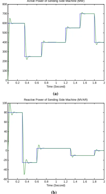
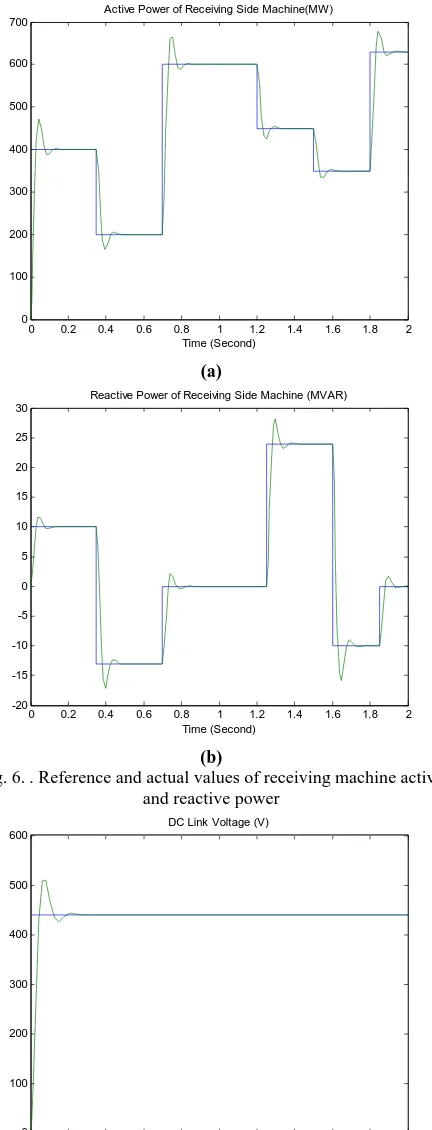
Fig.4-7 illustrate superior performance of feedback linearization scheme in asymptotically tracking of reference Signals. As is obvious in mentioned figures, each of outputs only needs a very short time(less than 0.2 second) to cope with the sudden change of their reference signal and settle on the references values. In Fig 5. it is illustrated that even in worst case in which three phase ground fault is occurred, the proposed nonlinear control, have the powerful ability to compensate it almost as soon as the faulty condition vanishes. In other word, in the post fault condition the proposed nonlinear control scheme exhibits a superior

compensating function. At the last it is worth to say such a fast, and exponential convergent performance that in addition has a good transient response could never be achieved with any linear control. Meanwhile the independent operating point performance of the proposed nonlinear control is clearly illustrated in Fig. 5 in which a large disturbance terribly changes the operating condition of system.

VI. CONCLUSION

In this paper the state space modeling and nonlinear control design of C-UPFC as an elegant FACTS device are presented. It was shown that with proposed nonlinear control scheme, independent of operating point, C-UPFC can easily regulate and compensate line active and reactive power flows and DC link and magnitude of load bus ac voltage especially in transient modes in which linear control have many problems. Meanwhile the superior capability of C-UPFC for control more than four variables in power line system as an advantage in compare with UPFC was clarified. It was shown in the simulations results that the proposed nonlinear MIMO controller with the help of state space modeling, considerably improve the dynamic of response and exhibit almost full tracking, even for step

changing in the active and reactive power, in compare with

past published researches on power transmission system including C-UPFC.

REFERENCES

[1] L. Gyugi, "A unified power flow control concept for flexible ac

transmission systems", IEE Proc. Part C. 139 (4) 1992, 323–331

[2] N. Mithulananthan, "Application of FACTS Controllers in Thailand

Power Systems", RTG Budget-Joint Research Project, 2003. New York: Springer-Verlag, 1985, ch. 4.

[3] Julia.j.black, "Flexible AC Transmission System

Compensation on a Utility Transmission System", A Thesis for Degree of Master of science, University of Nevada, Las Vegas, December 1994

[4] Hingorani N.G. and L. Gyugui, "Understanding FACTS", IEEE Press,

New York, 2000.

[5] M. Vilathgamuwa, X. Zhu, S.S. Choi, “A robust control method to

Improve the performance of a unified power flow controller” Electric Power Systems Research 55 (2000) 103–111

[6] Juan M.Ramirez , Ricardo J.Davalos , Abraham Valenzuela ,

Ixtlahuatl Coronado, , "FACTS-BasedStabilizers Coordination"

Trans.1995, pwrd,10(2): 1085-109.

[7] Gyugyi L. and C.D. Schauder, "The Unified Power Flow Controller: a

New Approach to Power Transmission Control", IEEETrans.1995,

pwrd,10(2): 1085-109.

[8] A.j.Keri, A.A.Edris, "Unified Power Flow Controller: Modeling and

Analysis",IEEE Trans, 1999

[9] H.F.Wang, "A Unified Model for the Analysis of FACTS Devices in

Damping Power System Oscillations Part I: Single-machine Infinite-bus Power Systems", IEEE Trans on Power Delivery, 1997

[10] S.A. Taher, " Design of Robust UPFC Controller Using H_ Control

Theory in Electric Power System “American Journal of Applied

Sciences 5 (8): 980-989, 2008

[11] Boon Teck Ooi, Bin Lu, “C-UPFC: A New FACTS Controller with 4

Degrees of Freedom”, 0-7803-5692-6, 2000 IEEE

[12] B. Ooi, B. Lu, “C-UPFC: A new FACTs Controller for Midpoint

Sitting”, Conf.Record of the Int. Power Electron.. Conf., April, 2000,Tokyo, Japan, pp. 1947– 1952

[13] A. Ajami , S.H. Hosseini , S. Khanmohammadi , G.B. Gharehpetian

"Modeling and Control of C-UPFC for Power System Transient Studies, Simulation Modeling Practice and Theory 14 (2006) (564– 576)

[14] Nabavi-Niakani. A., and Iravani. M.R, ‘Steady-State and Dynamic

Models of Unified Power Flow Controller (UPFC) for Power System

Studies”, IEEE Trans.,1996, PWRW, pp.1937-1943

[15] J.J.E.Slotine, "Applied Nonlinear Control", 1991 by Prentice Hall Inc,