Capturing the Process Efficiency and Congestion
of Supply Chains
Mithun J. Sharma & Yu, Song Jin
∗Abstract— This paper examines the performance of supply chain in stages keeping the essence of processes that knits the stages of supply chain. By focusing on the process as the unit of analysis, the management of inter-organizational relations in a way which is gen-erally known as network, on performance is analyzed. In order to enhance and extend the variation of date envelopment analysis (DEA) methodology, this paper serves to supplement the DEA literature in its ap-plication to supply chain retail sector. In addition an examination of input congestion is carried out in-dicates that a managerial inefficiency exist in the dif-ferent process cycles of supply chains. However, pres-ence of congestion indicates the inability to dispose of unwanted inputs costlessly. Using the DEA vari-ation of the supply chains are partitioned into three levels/stratums namely ’best-in-class’, ’average’ and ’laggard’. Substantial performance inefficiency is un-covered in the four process cycle dimensions. Rela-tively down-stream process cycles of the supply chain exhibit better performance than the up-stream pro-cess cycles. Our innovative approach identifies areas for improved supply chain performance over the four
process cycles. The classification of supply chains
serve as a guideline for best practices, and projects directly to the best class.
Keywords: supply chain, DEA, congestion, process cy-cles
1
Introduction
A major sintered and fiction building product manufac-turer achieved a $2 million saving in raw material cost by leveraging its purchase volume, obtaining a marginally lower unit price for an automobile type raw material, and changing suppliers. Six months later, a study of manufac-turing efficiency found that the new supplier’s material reduced finished products yield and increased product re-work rates that translated into reduced customer in-stock levels. The over-all effect? About $4.5 million cost to the
∗This research was a part of the results of the project called ” In-ternational Exchange & Cooperation Project for Shipping, Port & International Logistics” funded by the Ministry of Land, Transport and Maritime Affairs, Government of South Korea. (Manuscript submitted: 11/03/2010), * Corresponding author, Division of Ship-ping Management, Korea Maritime University, Busan, South Ko-rea, Tel/Fax: +82 51 410 4383 Email: [email protected] & Centre for Management Studies, Dibrugarh University, Dibrugarh, Assam, India, Tel/Fax: +91 373 2101423; [email protected]
overall bottom line. In this case the action was in line with the performance measure that had been established for purchasing department, yet the company was worse off overall. By each player in the supply chain acting in-dependently to meet its own performance measures, the result is duplicate inventories, ineffective promotions, ex-cess handling and poor new product introduction prac-tices that add significant cost to consumers and reduce the profitability of everyone involved in the chain. If you only manage your department from within the four-walls, you end up with a balloon effect that cripples your busi-ness.
first step towards improvement.
Performance measurement plays an essential role in eval-uating production because it can define not only the cur-rent state of the system but also its future. According to Dyson[11], performance measurement helps move the system in the desired direction through the effect exerted by the behavioral responses towards these performance measures that exist within the system. Mis-specified per-formance measures, however, will cause unintended con-sequences, with the system moving in the wrong direction [11]. The underlying assumption behind this claim is the role or presence of drivers such as effciency and effec-tiveness in the composition of performance. To put it in a simple way, effciency in Dyson’s [11] claim is ’doing things right’ and effectiveness is ’doing the right thing’. The combination of these two key drivers helps move the system in the right direction by doing the right thing. The definition of performance/performance management revolves around key concepts like efficiency and effective-ness. Let’s take a simple example of two car manufactur-ing companies to distmanufactur-inguish the two concepts. Suppose one of the firms produces car for the market and it does
it right without any slacks1, with optimal utilization of
resources relative to the other firm, we can label that firm as efficient however we cannot label it as effective. Effectiveness is the degree to which the outputs of a firm achieve the stated objectives of that service for exam-ple, the extent to which the firm is meeting the customer demand for a sedan or different car models. The effi-cient firm in the example may not be necessarily effective or an inefficient firm on the other hand may be effective and vice versa. Thus efficiency is the degree to which the observed use of resources to produce outputs of a given quality matches the optimal use of resources to produce outputs of a given quality. This can be assessed in terms of technical efficiency and allocative efficiency. Efficiency, by its description, is reactive. It cannot be pro-active. It has to be measurable but what happens in the future is not measurable. Efficiency has to be more historical[6]. The future strategy of a firm is formulated based on the efficiency results of past and present.
Supply chain falls in the domain of production manage-ment which includes series of activities such as product design, forecasting, organizing physical facilities, quality control, plant maintenance, materials management and the like. All these activities need to be organized and implemented that the firm should realize increased pro-ductivity. Productivity refers to the amount of goods and services produced with the resources used. Productivity is measured with the help of a formula which is as follows:
P roductivity= Amount of goods producedAmount of resources used
1The extra amount by which an input (output) can be reduced
(increased) to attain technical efficiency after all inputs (outputs) have been reduced (increased) in equal proportions to reach the production frontier
Productivity and efficiency are closely related however there is a difference between the two concepts. The in-dices of productivity is an absolute concept, measured by the ratio of amount of output to amount of resources whereas the efficiency indices is a relative concept, mea-sured by comparing the actual ratio of amount of output to amount of resources with optimal ratio of output to input.
The efficiency is determined by using a variation of frontier estimation especially data envelopment analysis (DEA) amidst multiple inputs and outputs. In particular, DEA methodology has proved to be powerful for bench-marking and identifying efficient frontiers especially for single producers or decision making units (DMU). Litera-ture reviews, such as the excellent bibliography in Seiford [20], reveal that research examining the use of mathemat-ical programming and associated statistmathemat-ical techniques to aid decision-making in supply chain benchmarking is
lacking. Liang et al.[16] points out that traditionally
most models (deterministic and stochastic) dealt with isolated parts of supply chain systems. Liang et al.[16] developed a Stackelberg co-operative model to evaluate the efficiency of SC members using DEA but their study was neither empirical nor showed any relationship of co-operation among members. An empirical study to eval-uate the efficiency of whole supply chain was done by Reiner and Hoffman[18]. They tried to evaluate the pro-cesses in a supply chain using the performance measure
of SCOR2, however they considered various processes of
a single supply chain instead of multiple chains. This leaves us with a literature gap and a question on how to measure the performance of supply chain considering each supply chain as meta-DMU. Research is required to find out how to measure the efficiency of a supply chain keeping an eye on key performance metrics that can cover all the interfaces in a supply chain. Usually the supply chain is evaluated in a sequential order:
Suppliers →Manufacturer →Distributor →Retailer → Consumer
Some researchers have tried to evaluate the chain in a serial order. Some of them tried to use a single perfor-mance measure e.g. (Cheung and Hausman[9]). Others like Chen and Zhu[7] provided two approaches in model-ing efficiency as a two-stage process. Golany et. al.[15] provided an efficiency measurement framework for sys-tems composed of two subsyssys-tems arranged in series that simultaneously compute the efficiency of the aggregate system and each subsystem. Zhu[22], on the other hand, presented a DEA-based supply chain model to define and measure the efficiency of a supply chain and that of its members. Fare and Grosskopf[13] and Castelli et al[4] in-troduced the network DEA model, in which the interior structure of production units can be explicitly modeled.
2Supply-Chain Operations Reference model. c.f. [19] for some
However, a supply chain is a sequence of processes and flows that take place within and between different stages and combine to fill a customer need for a product. The objective of every supply chain is to maximize the overall value generated. The value a supply chain generates is the difference between what the final product is worth to the customer and the effort the supply chain expends in filling the customer’s request. For most commercial
supply chains, value will be strongly correlated with
sup-ply chain profitability. Supply chain profitability is the total profit shared across all the supply chain stages [8]. All the above mentioned studies evaluated supply chain in stages ignoring the essence of processes that knits the stages of supply chain. By focusing on the process as the unit of analysis, the management of inter-organizational relations in a way which is generally known as network, on performance is analyzed. In order to enhance and extend the variation of DEA methodology this paper serves to supplement the DEA literature in its applica-tion to supply chain retail sector. Using the DEA vari-ation of [21] the supply chains are partitioned into three levels/stratums namely ’best-in-class’, ’average’ and ’lag-gard’ [1]. In addition an examination of input congestion is carried out indicates that a managerial inefficiency [10] exist in ’average’ and ’laggard’ supply chains. By simply reconfiguring this excess resources it may be possible to increase output without reducing the inputs. Equipped with this knowledge, managers will be better able to de-termine when large reengineering projects are necessary versus minor adjustments to existing business processes. The supply chain process cycles and performance eval-uation is discussed in Section 2 followed by our object-oriented DEA models and the resulting empirical findings in Section 3. Finally, Section 4 summarizes and concludes the paper.
2
Processes in Supply Chain
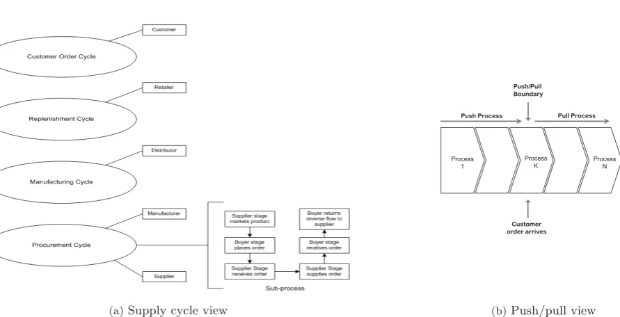
As already mentioned at the outset, a supply chain is a sequence of processes and flows that take place within and between different stages and combine to fill a cus-tomer need for a product with an objective to maximize the overall value of the supply chain. Previous studies evaluated supply chain in stages ignoring the essence of processes that knits the stages of supply chain. Therefore evaluating supply chain processes and subprocesses will help to effectively analyze supply chain as a whole. Dav-enport and Short (1990) define ‘processas a set of logically related tasks performed to achieve a defined business out-come and suggest that processes can be divided into those that are operationally oriented (those related to the prod-uct and customer) and management oriented (those that deal with obtaining and coordinating resources). There are two different ways to view the processes performed in a supply chain.
• Cycle View: The processes of a supply chain are
divided into a series of cycles, each performed at the interface between two successive stages of a supply chain
• Push/pull view: The processes in a supply chain are
divided into two categories depending on whether they are executed in response to a customer order or in anticipation of customer orders.
A cycle view of the supply chain clearly defines the pro-cesses involved and the owners of each process. This view is very useful when considering operational decisions be-cause it specifies the roles and responsibilities of each member of the supply chain and the desired outcome of each member of the supply chain and the desired out-come for each process. While the push/pull view of the supply chain categorizes processes based on whether they are initiated in response to a customer order (pull) or in anticipation of a customer order (push). This view is use-ful when considering the strategic decisions. A schematic representation of both the processes are shown in figure 1.
Let’s consider the cycle view of supply chain processes. Given the five stages of a supply chain, all supply chain processes can be broken down into four process cycles as shown in figure 1(a). Each cycle occurs at the interface between two successive stages. The five stages thus result in four supply chain process cycles. Each cycle consist of processes again shown in figure 1(b). These sub-processes may vary from industry to industry. We now describe the various supply chain cycles comprehensively in the subsequent sub-sections.
2.0.1 Customer Order Cycle
The customer order cycle [8] occurs at the cus-tomer/retailer interface and includes all processes di-rectly invloved in receiving and filling the customer’s or-der. Typically, the customer initiates this cycle at a re-tailer site and the cycle primarily involves filling customer
demand. The retailer’s interaction with the customer
starts when the customer receives the order. The pro-cesses involved in the customer order cycle are shown in Figure 1(b) and include:
• Customer arrival
• Customer order entry
• Customer order fulfillment
• Customer order receiving
(a)Supply cycle view
Push Process Pull Process Push/Pull
Boundary
3URFHVV 1 3URFHVV
. 3URFHVV
Customer order arrives
[image:4.595.36.482.94.322.2](b)Push/pull view
Figure 1: Process views of a supply chain: There are two different ways to view the processes performed in a supply chain. Figure (a) Cycle view of supply chain processes (b) Push/pull view of supply chain processes. Cycle view is important when considering operational decisions and push/pull view for strategic decision.
and makes a decision regarding a purchase. Customer arrival can occur when the customer walks into a super-market to make a purchase. The goal in this process of customer’s arrival is to facilitate an appropriate product so that the customer’s arrival turns into a customer or-der. At a retail super mall a customer order may involve managing customer flows and product displays. The ob-jective of the customer arrival process is to maximize the conversion of customer arrivals to customer orders.
Customer order entry: The customer order entry refers to customers informing the retailer what products they want to purchase and the retailer allocating product to customer. At a super mall, order entry may take the form of customers loading all items that they intend to purchase into their carts.
Customer order fulfillment: During this process, the cus-tomer’s order is filled and sent to the customer. At a super mall, the customer performs this process. In gen-eral, customer order fulfillment takes place from retailer inventory.
Customer order receiving: During this process, the cus-tomer receives the order and takes ownership. Records of this receipt may be updated and payment completed. At a super mall, receiving occurs at the checkout counter.
Given the five supply chain stages
(supplier-manufacturer-distributor-retailer-customer), all supply chain processes are divided into four process cycles and the factors are expressed as inputs and outputs in each
cycle. In the first cycle i.e. thecustomer order cycle in
a retail setting, the customer walks into a supermarket
to make purchase. The manager may group similar
merchandise enabling customers to find desired items easily (a process layout). At the same time, the layout often leads customers along predetermined paths such as up and down aisles (a product layout). With this hybrid layout of the retail mart, the customer chooses his/her product and ends with customer receiving the product.
Hence, in this cycle the inputs identified are -
tech-nological functionality, sales order by FTE (Full-Time Employee) and the outputs are - order fulfillment cycle time,customer check-out time. The data categories that are used for analysis in customer order process cycle are described in table 1.
Table 1: Inputs/outputs of customer order process cycle
Inputs
Technological
func-tionality
The functionality of the technology in place. This is measured in units of functionality where a higher number indicates more functionality.
Sales order by FTE This indicator measures the number
of customer orders that are processed by full time employees per day.
Outputs
Order fulfillment cy-cle time
It is a continuous measurement de-fined as the amount of time from cus-tomer authorization of a sales order to the customer receipt of product
Cycle inventory It represents the average order
[image:4.595.296.570.578.769.2]Supply Cycle 1
Supply Cycle 2
Supply Cyclem
Sub-process 1 Sub-process 2 …….. Sub-process n
Inputs/outputs Inputs/outputs Inputs/outputs
Inputs/outputs Inputs/outputs Inputs/outputs
Inputs/outputs Inputs/outputs Inputs/outputs
…….. …….. ……..
Efficiency score of sub-process 2
Efficiency score of sub-processn Efficiency score of
sub-process 1
……..
……..
(a)Sub-process evaluation
Supply Cycle 1
Supply Cycle 2
Supply Cyclem
Sub-process 1 Sub-process 2 …….. Sub-process n
Inputs/outputs Inputs/outputs Inputs/outputs
Inputs/outputs Inputs/outputs Inputs/outputs
Inputs/outputs Inputs/outputs Inputs/outputs
…….. …….. ……..
Efficiency score of whole supply chain processes
……..
[image:5.595.31.555.137.324.2](b)Meta-process evaluation
Figure 2: Figure (a) Sub-process evaluation in each supply chain process cycle (b) Schematic for evaluating the meta-process efficiency of supply chains
2.0.2 Replenishment Process Cycle
The replenishment process cycle [8] occurs at the re-tailer/distributor interface and includes all processes in-volved in replenishing retailer inventory. It is initiated when a retailer places an order to replenish inventories to meet future demand. A replenishment cycle may be triggered at a supermarket that is running out of stock of a particular product e.g. detergent. The replenishment cycle is similar to customer order process cycle except that the retailer is now the customer. The processes in-volved in the replenishment cycle include:
• Retail order trigger
• Retail order entry
• Retail order fulfillment
• Retail order receiving
Retail order trigger: As the retailer fills customer de-mand, inventory is depleted and must be replenished to
meet future demand. A key activity the retailer
per-forms during the replenishment cycle is to devise a re-plenishement or ordering policy that triggers and order from the previous stage. The objective when setting re-plenishment order triggers is to maximize profitability by ensuring economies of scale and balancing product avail-ability and cost of holding inventory. The outcome of the retail order trigger process is the generation of a re-plenishment order that is ready to be passed on to the distributor or manufacturer.
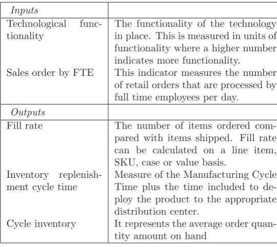
Table 2: Inputs/outputs of replenishment process cycle
Inputs
Technological
func-tionality
The functionality of the technology in place. This is measured in units of functionality where a higher number indicates more functionality.
Sales order by FTE This indicator measures the number
of retail orders that are processed by full time employees per day.
Outputs
Fill rate The number of items ordered
com-pared with items shipped. Fill rate can be calculated on a line item, SKU, case or value basis.
Inventory
replenish-ment cycle time
Measure of the Manufacturing Cycle Time plus the time included to de-ploy the product to the appropriate distribution center.
Cycle inventory It represents the average order
quan-tity amount on hand
[image:5.595.296.567.404.645.2]Retail order fulfillment: This process is similar to cus-tomer order fulfillment except that it takes place at the distributor. A key difference is the size of each order as the customer order tend to be much smaller than the replenishment orders.
Retail order receiving: Once the replenishment order ar-rives at a retailer, the retailer must receive it physically and update all inventory records. This process involves product flow from the distributor to the retailer as well as information updates at the retailer and the flow of funds form the retailer to the distributor.
In replenishment process cycle the inputs identified are - Technological functionality, sales order by FTE (Full-Time Employee) and the outputs identified are - fill rate, inventory lead time, and cycle inventory. The data cate-gories that are used for analysis in replenishment process cycle are described in table 2.
2.0.3 Manufacturing Cycle
The manufacturing cycle [8] occurs at the distrib-utor/manufacturer (or retailer/manufacturer) interface and includes all processes involved in replenishing retailer inventory. The manufacturing cycle is triggered by cus-tomer orders/replenishment orders/forecast of cuscus-tomer demand and current product availability in the manufac-turer’s finished goods warehouse. The processes involved in the manufacturing cycle are shown in figure 1(b) and include:
• Order arrival
• Production scheduling
• Manufacturing and shipping
• Receiving at distributor, retailer or customer
Order arrival: During this process, a finished-goods warehouse or distributor sets a replenishment order trig-ger based on the forecast of future demand and current product inventories. This process is similar to the retail order trigger process in the replenishment cycle.
Production scheduling: During the production scheduling process, orders are allocated to a production plan. Given the desired production quantities for each product, the manufacturer must decide on the precise production
se-quence. The demand for a finished good tends to be
independent and relatively stable. However, firms typi-cally make more than one product on the same facilities, so production is generally done in lots. The quantities and delivery items needed to make those end items are
determined by the production schedule. More
[image:6.595.302.568.127.445.2]specifi-cally, materials requirement planning (MRP) explosion
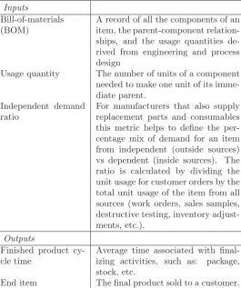
Table 3: Inputs/outputs of manufacturing process cycle
Inputs
Bill-of-materials (BOM)
A record of all the components of an item, the parent-component relation-ships, and the usage quantities de-rived from engineering and process design
Usage quantity The number of units of a component
needed to make one unit of its imme-diate parent.
Independent demand ratio
For manufacturers that also supply replacement parts and consumables this metric helps to define the per-centage mix of demand for an item from independent (outside sources) vs dependent (inside sources). The ratio is calculated by dividing the unit usage for customer orders by the total unit usage of the item from all sources (work orders, sales samples, destructive testing, inventory adjust-ments, etc.).
Outputs
Finished product cy-cle time
Average time associated with
final-izing activities, such as: package,
stock, etc.
End item The final product sold to a customer.
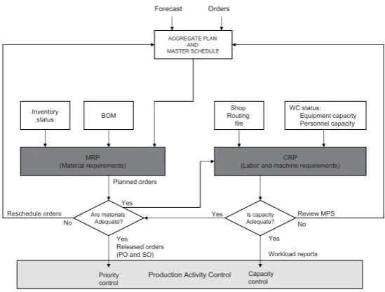
andcapacity requirement planning (CRP)are used. MRP explosion converts the requirements of various final prod-ucts into a material requirements plan that specifies the replenishment schedules of all the sub assemblies, com-ponents and raw materials needed by the final product. Whereas, CRP is the process of determining what person-nel and equipment capacities are needed to meet the pro-duction objective embodied in the master schedule and material requirement plan. Figure 3 describes MRP and CRP activities in schematic form. Forecasts and orders are combined in the production plan, which is
formal-ized in themaster production schedule (MPS). The MPS,
along with a bill-of-material (BOM) file and inventory
status information, is used to formulate the MRP. The MRP determines what components are needed and when they should be ordered from and outside vendor/supplier or produced in-house. The CRP function translates the MRP decisions into hours of capacity (time) needed. If material, equipments and personnel are adequate, orders are released and the workload is assigned to the various work stations.
AGGREGATE PLAN AND MASTER SCHEDULE
WC status: Equipment capacity Personnel capacity Shop
Routing file BOM
Inventory status
MRP (Material requirements)
CRP (Labor and machine requirements)
Are materials Adequate?
Is capacity Adequate?
Production Activity Control Forecast Orders
Yes Released orders (PO and SO)
Yes
Workload reports
Priority control
Capacity control Yes
No Review MPS Yes
No Reschedule orders
[image:7.595.154.429.103.311.2]Planned orders
Figure 3: Material and capacity planning flowchart
process, the product is shipped to the customer, retailer, distributor, or finished-product warehouse.
Receiving: In this process, the product is received at the distributor, finished-goods warehouse, retailer, or cus-tomer and inventory records are updated. Other pro-cesses related to storage and fund transfer also take place.
In manufacturing process cycle the inputs identified are - bill-of-materials (BOM), usage quantity, Independent demand ratio, and the outputs identified are - Finished product cycle time, end item. The data categories that are used for analysis in replenishment process cycle are described in table 3.
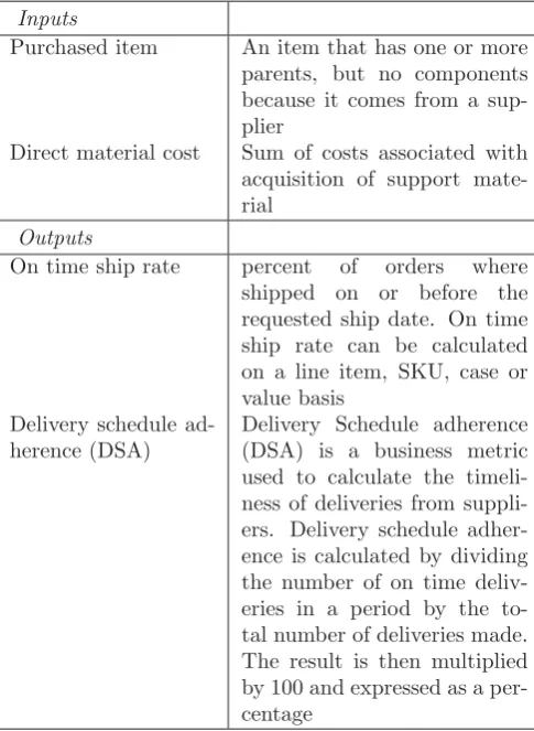
2.0.4 Procurement Cycle
The procurement cycle [8] occurs at the manufac-turer/supplier interface and includes all processes nec-essary to ensure that materials are available for man-ufacturing to occur according to schedule. During the procurement cycle, the manufacturer orders componenets from suppliers that replenish the component inventories. The relationship is quite similar to that between a dis-tributor and manufacturer with one significant difference. Wheras retailer/distributor orders are triggered by uncer-tain customer demand, components orders can be deter-mined precisely once the manufacturer has decided what the production schedule will be. In practice, there may be several tiers of suppliers, each producing a component for next tier. A similar cycle would then flow back from one stage to the next. The processes of procurement cycle are shown in figure 1(b). In procurement process cycle
the inputs identified are - Purchased item, Direct
Mate-rial Cost, and the outputs identified are - On time ship rate,Delivery Schedule Adherence (DSA). The data cate-gories that are used for analysis in replenishment process cycle are described in table 4.
The evaluation of efficiency of sub-processes is performed by inputs and outputs of each supply chain process cy-cle. After collecting data of inputs and outputs of pro-cesses, efficiency of each sub-process will be evaluated using DEA. Figure 2(a) shows the structure of
evaluat-ing efficiency of a supply chain sub-process which hasm
cycles (usually there will be four cycles but in some
in-dustry there may be less, e.g. Dell, Amazon etc.) withn
sub-processes in each supply chain. Here we have shown just one sub-process of a single cycle however there will be many sub-processes in each supply cycle. Therefore at this stage, computations of efficiency are executed as many times as the number of sub-processes in the chain, as efficiency is evaluated at the process-level. In case of
figure 2(a), there arenresults of sub-process efficiency in
each supply cycle.
2.0.5 Evaluating overall efficiency of a supply chain
Table 4: Inputs/outputs of procurement process cycle
Inputs
Purchased item An item that has one or more
parents, but no components because it comes from a sup-plier
Direct material cost Sum of costs associated with
acquisition of support mate-rial
Outputs
On time ship rate percent of orders where
shipped on or before the
requested ship date. On time ship rate can be calculated on a line item, SKU, case or value basis
Delivery schedule ad-herence (DSA)
Delivery Schedule adherence (DSA) is a business metric used to calculate the timeli-ness of deliveries from suppli-ers. Delivery schedule adher-ence is calculated by dividing the number of on time deliv-eries in a period by the to-tal number of deliveries made. The result is then multiplied by 100 and expressed as a per-centage
through a pure output DEA model suggested by Lovell and Pastor [17]. With the DEA model, the weights of each sub-process can be included in evaluating the over-all efficiency of a supply chain. Unlike a simple aggrega-tion of processes efficiency, it considers relative impacts of processes on supply chains efficiency (refer to Figure 3 for illustration). It will use efficiency scores of each pro-cess as values of output in order to assess the efficiency of a supply chain. In the case of Figure 2(b), each
sup-ply cycle will have the efficiency scores ofnsub-processes
and the whole supply chain has the overall efficiency of
m supply cycles. Thus this aggregate efficiency of
sup-ply chain will be considered as single DMU. In a similar vein, different supply chains of a particular industry will be analyzed.
3
Measuring Process Efficiency and
Con-gestion of each Process Cycle
There are some issues related to measuring the efficiency of a supply chain using DEA. The first is supply chain operations involve multiple inputs and outputs of dif-ferent forms at different stages and second is that the performance evaluation and improvement actions should
be coordinated across all levels of production in a
sup-ply network. In this paper, we evaluate supply chain
stages in process cycles keeping the essence of processes that knits the stages of supply chain. By focusing on the process as the unit of analysis, the management of inter-organizational relations in a way which is generally known as network, on performance will be analyzed.
DEA models are classified with respect to the type of envelopment surface, the efficiency measurement and the orientation (input or output). There are two basic types of envelopment surfaces in DEA known as con-stant returns-to-scale (CRS) and variable returns-to-scale (VRS) surfaces. Each model makes implicit assumptions concerning returns-to-scale associated with each type of surface. Charnes et al.[5] introduced the CCR or CRS model that assumes that the increase of outputs is pro-portional to the increase of inputs at any scale of op-eration. Banker et al.[2] introduced the BCC or VRS model allowing the production technology to exhibit in-creasing scale (IRS) and dein-creasing returns-to-scale (DRS) as well as CRS.
3.0.6 The BCC Model
The input-oriented BCC model evaluates the efficiency ofDM Uo(o= 1, ..., n) by solving the following envelop-ment form:
(BCCo)
minθB,λθB
subject toθBxo−Xλ≥0
Y λ≥yo
eλ≥0,
whereθB is a scalar
The dual multiplier form of this linear program (BCCo)
is expressed as
maxv,u,uoz=uyo−uo
subject tovxo= 1
−vX+uY −uoe≤0
v≥0, u≥0, uo free in sign,
where, v and u are vectors and z and uo are scalars
and the latter, being ’free in sign,’ may be positive or negative or zero. The equivalent BCC fractional program is obtained from the dual program as:
maxuyo−uo vxo
subject to uyj−uo
vxj ≤1 (j= 1, ..., n)
v≥0, u≥0,uo free.
The primal problem (BCCo) is solved using two-phase
second phase, we maximize the sum of the input excesses
and output shortfalls, keeping θB = θB∗. An optimal
solution for (BCCo) is represented by θB∗, λ∗, s−∗, s+∗,
wheres−∗ ands+∗ represent the maximal input excesses
and output shortfalls, respectively.
BCC-Efficiency: If an optimal solutionθ∗B, λ∗, s−∗, s+∗
obtained in this two phase process for (BCCo) satisfies
θ∗B= 1
and has no slacks (s−∗ = 0 ands+∗ = 0), then theDM Uo
is called BCC-efficient, otherwise it is BCC-inefficient.
Reference Set: For a BCC-inefficientDM Uo, we define
its reference set,Eo, based on an optimal solutionλ∗by
Eo=
j|λ∗j ≥0
(j∈ {1, ..., n})
If there are multiple optimal solutions, we can choose any one to find that
θ∗Bxo=
j∈Eo
λ∗jxj+s−∗
yo=
j∈Eo
λ∗jyj−s+∗
Thus the improvement path via the BCC projection,
ˆ
xo⇐θ∗Bxo−s−∗ ˆ
[image:9.595.300.498.590.747.2]yo⇐yo+s+∗
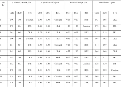
Figure 4 shows the efficiency results of the CCR and BCC model for 11 supply chain sub-processes of a partic-ular product (e.g. detergent). First, the efficient supply chains, in each process cycle are: customer order cycle (1, 4, 7, 9, and 11) replenishment cycle (1, 2, 5, 6, 8, 11), manufacturing cycle (2, 4, 6) and procurement cycle (5, 6, 9). The same figure shows the efficiency results of RTS. The RTS efficiency score is calculated as the ratio of a CCR efficiency score to a BCC efficiency score. Figure 4 indicates that, customer order cycle, the BCC efficient but not scale-efficient process cycles were operating on an IRS frontier. For customer order cycle, five BCC-efficient retail chains were operating on IRS and four on DRS fron-tiers. Of the BCC-inefficient supply chains, 64% and 20% were in the IRS region in cycle 1 and cycle 2, respectively. As economists have long recognized, an IRS frontier firm would generally be in a more favorable position for ex-pansion, compared to a firm operating in a CRS or DRS region. Note that the concept of RTS may be ambiguous unless a process cycle is on the BCC-efficient frontier, since we classified RTS for inefficient process cycles by their input oriented BCC projections. Thus, a different
RTS classification may be obtained for a different orien-tation, since the input-oriented and the output-oriented BCC models can yield different projection points on the VRS frontier. Thus, it is necessary to explore the ro-bustness of the RTS classification under the output ori-ented DEA method. Note that an IRS DMU (under the output-oriented DEA method) must be termed as IRS by the input oriented DEA method. Therefore, one only needs to check the CRS and DRS banks in the current study. Using the input-oriented approach, we discover that only two DRS supply chains in replenishment cycle (DMUs 2, 4, 6 and 9) and seven DRS (DMUs 1, 3, 4, 5, 6, 7, and 9) in the manufacturing cycle. These results indicate that (i) in general, the RTS classification under different process cycle is independent of the orientation of DEA model; and (ii) there are serious input deficiencies in manufacturing cycle3 at the current usage quantities derived from engineering and process design.
3.1
Input Congestion in Supply Chains
Congestion is said to occur when the output that is max-imally possible can be increased by reducing one or more inputs without improving any other input or output. Conversely, congestion is said to occur when some of the outputs that are maximally possible are reduced by in-creasing one or more inputs without improving any other input or output. For example, excess inventory clutter-ing a factory floor in a way that interferes with
produc-tion. By simply reconfiguring this excess inventory it
may be possible to increase output without reducing in-ventory. This improvement represents the elimination of inefficiency that is caused by the way excess inventory is managed. There are many models dealing with conges-tion but we start with FGL (Fre, Grosskopf and Lovell 1985, 1994) because it has been the longest standing and most used approach to congestion in the DEA literature.
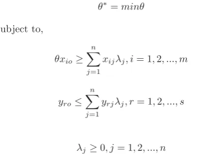
Fare, Grosskopf and Lovell (FGL) approach proceeds in two stages. The first stage uses an input oriented model as follows (Fare et al.[12]):
θ∗=minθ
subject to,
θxio≥ n
j=1
xijλj, i= 1,2, ..., m (1)
yro≤ n
j=1
yrjλj, r= 1,2, ..., s
λj≥0, j= 1,2, ..., n
where j = 1, ..., n indexes the set of DMUs (Decision
DMU ID
Customer Order Cycle Replenishment Cycle Manufacturing Cycle Procurement Cycle
CCR BCC RTS CCR BCC RTS CCR BCC RTS CCR BCC RTS
1 1.00 1.00 Constant 1.00 1.00 Constant 0.08 0.19 DRS 0.63 0.98 DRS
2 0.70 0.84 IRS 0.48 1.00 IRS 1.00 1.00 Constant 0.73 0.84 IRS
3 0.45 0.49 DRS 0.76 0.82 IRS 0.06 0.09 DRS 0.17 0.18 IRS
4 1.00 1.00 Constant 0.45 0.61 IRS 0.46 1.00 DRS 0.64 0.92 DRS
5 0.51 0.54 IRS 1.00 1.00 Constant 0.13 0.39 DRS 0.44 1.00 DRS
6 0.43 0.62 IRS 0.66 1.00 IRS 0.27 1.00 DRS 0.64 1.00 DRS
7 0.97 1.00 DRS 0.69 0.70 DRS 0.02 0.03 DRS 0.12 0.12 IRS
8 0.52 0.53 IRS 1.00 1.00 Constant 0.10 0.10 Constant 0.28 0.30 IRS
9 0.90 1.00 IRS 0.45 0.95 IRS 0.43 0.75 DRS 1.00 1.00 Constant
10 0.74 0.94 DRS 1.00 1.00 Constant 0.01 0.02 IRS 0.09 0.11 IRS
[image:10.595.90.499.97.396.2]11 0.76 1.00 DRS 0.96 1.00 DRS 0.01 0.02 IRS 0.06 0.07 IRS
Figure 4: CCR, BCC and RTS results
DMU ID
Customer Order Cycle Replenishment Cycle Manufacturing Cycle Procurement Cycle
1 1.00 1.00 1.00 1.00 1.00 1.00 0.19 0.19 1.00 0.98 0.98 1.00
2 0.84 0.84 1.00 0.98 1.00 0.98 1.00 1.00 1.00 0.79 0.84 0.94
3 0.45 0.49 0.91 0.80 0.82 0.97 0.06 0.09 0.66 0.17 0.18 0.94
4 1.00 1.00 1.00 0.61 0.61 1.00 0.87 1.00 0.87 0.92 0.92 1.00
5 0.51 0.51 1.00 1.00 1.00 1.00 0.31 0.39 0.79 0.66 1.00 0.66
6 0.60 0.62 0.96 0.66 1.00 0.66 0.77 1.00 0.77 1.00 1.00 1.00
7 0.97 1.00 0.97 0.69 0.70 0.98 0.02 0.03 0.66 0.12 0.12 1.00
8 0.52 0.53 0.98 1.00 1.00 1.00 0.10 0.10 1.00 0.28 0.30 0.93
9 1.00 1.00 1.00 0.95 0.95 1.00 0.75 0.75 1.00 1.00 1.00 1.00
10 0.74 0.74 1.00 1.00 1.00 1.00 0.02 0.02 1.00 0.10 0.11 0.90
11 0.76 0.76 1.00 0.96 1.00 0.96 0.02 0.02 1.00 0.07 0.07 1.00 *
T
*E
**T E
*
T
*T
*T
*
E
*E
*E
** T E
*
* T E *
* T E
[image:10.595.87.503.440.746.2]amount of input i = 1, ..., m used by DM Uj and yro
is the observed amount of output r = 1, ..., s produced
by DM Uj. The xioand yro represent the amounts of
inputs i = 1, ..., m and outputs r = 1, ..., s associated
with DM Uo where, DM Uo is the DM Uj = DM Uo to
be evaluated relative to all DM Uj (including itself).
The objective is to minimize all of the inputs ofDM Uo
in the proportion θ∗ where, because the xio = xij and
yro = yrj for DM Uj = DM Uo appear on both sides
of the constraints, the optimal θ = θ∗ does not exceed
unity and the nonnegativity of the λj, xij, and yij
implies that the value of θ∗ will not be negative under
the optimization in (1). Hence,
0≤M inθ=θ∗≤1 (2)
We now have the following definition of technical effi-ciency and ineffieffi-ciency,
Technical efficiency is achieved byDM Uo if and only if
θ∗= 1
Technical inefficiency is present in the performance of
DM Uoif and only if 0≤θ∗<1
Next, FGL then go on to the following second stage model,
β∗=minβ
subject to,
βxio= n
j=1
xijλj, i= 1,2, ..., m (3)
yro≤ n
j=1
yrjλj, r= 1,2, ..., s
λj≥0, j= 1,2, ..., n
Note that the first i = 1, ..., m inequalities in (1) are
replaced by equations in (3). Thus slack is not possible in the inputs. The fact that only the output can yield non-zero slack is then referred to as weak disposal by
Fre et al.[12]. Hence, we have 0 =θ∗≤β∗. FGL use this
property to develop a measure of congestion,
0≤C(θ∗, β∗) = θ
∗
β∗ ≤1 (4)
Combining models (1) and (3) in a two-stage manner, FGL utilize this measure to identify congestion in terms of the following conditions,
(i) Congestion is identified as present in the performance
ofDM Uoif and only if
C(θ∗, β∗)<1 (5)
(ii) Congestion is identified as not present in the
perfor-mance ofDM Uo if and only ifC(θ∗, β∗) = 1
In figure 5, we focus on the points for DMUs 3, 6, 7, and 8, of customer order cycle which are the only ones that satisfy the conditon for congestion specified in equation (5). For DMUs 3, 6, 7, and 8 in the figure 5 and coupling this value we obtain cogestion efficiency as 0.91, 0.96, 0.97 and 0.98 respectively. Around 36% of the supply chains have exhibited input congestion under VRS technologies. The inputs technological functionality and sales order by FTE in a VRS technology shows the congestion of sales order by FTE is 18.36% of the corresponding technolog-ical functionality input level.
Around 45% of the supply chains have exhibited input congestion under VRS technologies in the replenishment process cycle. In the replenishment process cycle we focus on DMUs 2, 3, 6, 7, and 11. We obtain congestion effi-ciecies of 0.98, 0.97, 0.66, 0.98 and 0.96 for these supply chains. The inputs technological functionality and sales order by FTE same as the customer order cycle, in a VRS technology shows the congestion of sales order by FTE is 26.66% of the corresponding technological functionality input level.
In the manufacturing cycle, the focus DMU points are 3, 4, 5, 6 and 7 which are the ones that satisfy the condi-tions of congestion specified in equation (5). The con-gestion efficiencies for these DMUS are 0.66, 0.87, 0.79, 0.77, and 0.66 respectively. The inputs bill-of-materials (BOM), usage quantity, independent demand ratio shows congestion by 15.2%, 22.4%, and 2.5% respectively. The residual score in manufacturing cycle largely indicates the scope for efficiency improvements resulting from less effi-cient work practices and poor management, but also re-flect differences between operating environments in these five supply chains.
The DMUS 2, 3, 5, 8 and 10 of the procurement cycle exhibits the presence of congestion. The congestion effi-ciency for these supply chains are found to be 0.94, 0.94, 0.66, 0.93, and 0.90 respectively. The inputs purchased item shows congestion by 23.3% of the correspond input direct material cost.
Starting with input (in the form of technological function-ality, order by FTE, BOM, usage quantity, independent demand ration, purchased items, direct material cost) at x=0 the output, y, measured in fill rate, cycle inventory, inventory replenishment cycle time, finished product cy-cle time, end time, on time ship rate and DSA, can be
increased at an increasing rate untilxois reached at
out-putyo. This can occur, for instance, because an increase
in the technological functionality, usage quantity, pur-chased items makes it possible to perform tasks in a man-ner that would not be possible with a smaller number of
inputs. Fromxo to x1 however, total output continues
possible output is reached aty1. Using more input results
in a decrease from this maximum so that atx2 we have
y2< y1 andy1−y2 is the amount of output lost due to
congestion. Under congestion, the inability to dispose of unwanted inputs increases costs.
3.2
Classification of Supply Chains
We have identified best-practice/performance of various supply cycles in supply chains and examined their conges-tion. However, we have not classified the supply chains which is required for a step-wise improvement, otherwise not possible with the traditional DEA. To classify the set of supply chains, we modify the algorithm developed by [21] to segment the supply chains into three classes namely, best-in-class, average, and laggard chains. The modified algorithm is as follows:
Assume there are n DMUs, each with m inputs and s
outputs. We define the set of all DMUs as J1, J1 =
DM Uj, j= 1, ..., nand the set of efficient DMUs inJ1as
E1. Then the sequences ofJ1andE1are defined
interac-tively asJl+1=
Jl−
El where
El=
DM Up∈Jl|φlp=l,
and φl
p is the optimal value to the following linear
pro-gramming problem:
maxλi,φφlp=φ
s.t.
i∈F(Jl)
λixji−xjp≤0∀j
i∈F(Jl)
λiyki−φykp≥0∀k
λi ≥0, i∈F(Jl)
wherek= 1 to s,j = 1 to m,i= 1 to n,yki = amount
of output k produced by DM Ui∗; xjp = input vector
of DM Up, xji = amount of input j utilized by DM Ui;
ykp= output vector ofDM Up. i∈F(Jl) in other words
DM Ui∈Jl, i.e. F(.) represents the correspondence from
a DMU set to the corresponding subscript index set. The following algorithm accomplishes subsequent stra-tum.
Step 1: Setl = 1. Evaluate the entire set of DMUs,Jl,
to obtain the set,E1, of first-level frontier DMUs (which
is equivalent to classical CCR DEA model), i.e. when
l= 1, the procedure runs a complete envelopment model
on all n DMUs and E1 consists of all of the DMUs on
the resulting overall best-practice efficient frontier.
Step 2: Exclude the frontier DMUs from future DEA
runs and setJl+1=
Jl−
El
Step 3: IfJl+1 = 3El+l, then stop. Otherwise, evaluate
the remaining subset of inefficient DMUs,Jl+1, to obtain
the new best-practice frontierEl+1.
Stopping Rule: The algorithm stops whenJl+1= 3
El+l.
We analyzed the aggregated metrics of the companies us-ing the modified algorithm of [21] to determine whether their performance ranked as best-in-class (36%), average (27%), or laggard (37%). In addition to having common performance levels, each class also shared characterstics in four process cycles: (1) customer order cycle (balances customer demand with supply from manufacturers); (2) replenishment process cycle (Balances retailer demand with distributor fill rate); (3) manufacturing cycle (bal-ances the percentage mix of demand for an item from in-dependent (outside sources) vs in-dependent (inside sources) across all supply chain stages); (3) procurement process cycle (balances Delivery Schedule adherence (DSA) for the timeliness of deliveries from suppliers). The char-acterstics of these performance metrics serve as guideline for best practices, and correlate directly with best-in-class performance.
Based on the findings in figure 6 derived from the con-text dependent DEA algorithm (modified), the best-in-class supply chains reveal the optimal utilization of tech-nological functionality along with the use of state-of-art technology. The average and laggard supply chains on the other hand must upgrade their technological func-tionality towards fast, responsive, and structured sup-ply chains where customer responsiveness, and collab-oration are necessary ingredients for continued and re-lentless inventory, margin, working capital, and perfect order-related success.
Best-in-class supply chains processes sales order by full time employees 24 - 32% more than the average and lag-gard chain in the replenishment process cycle. As well as the fill rate and the time required to deploy the product to the appropriate distribution center is 28% higher than the average and laggard supply chains.
In the manufacturing cycle front the inventory optimiza-tion goals are well served by best-in-class chains. They work closely with their trading partners, including sup-pliers, distributor, and retailers to reduce the pressure of increased lead times and potentially lower inventory levels for the chain. Due to this close collaboration, the finished product cycle time (average time associated with analyz-ing activities, such as: package,stock, etc.) and end item (the final product sold to a customer) less relative to av-erage and laggard supply chains by 34.5%.
Best-in-Class (E1) Average (E2) Laggards (E3)
Classes of efficient chains in % 36 % 27 % 37 %
Customer Order Cycle
Balances customer demand with supply from manufacturers
66 % 53 % 48 %
Replenishment Process Cycle
Balances retailer demand with distributor fill rate
55 % 31 % 23 %
Manufacturing Cycle
Balances the percentage mix of demand for an item from independent (outside sources) vs dependent (inside sources) across all supply chain stages
65 % 44 % 36 %
Procurement Process Cycle
Balances Delivery Schedule adherence (DSA) for the timeliness of deliveries from suppliers.
[image:13.595.86.499.100.405.2]52 % 48 % 45 %
Figure 6: Results of stratified supply chains
timeliness of deliveries from suppliers) in the procurement cycle does not show any significant difference among the best-in-class, average and laggard supply chains. There is only a 5% difference in the perfomance of this supplier manufacturer interface.
4
Conclusion
This paper analyzes the process cycles of 12 supply chains using an innovative DEA model. Close to 45% of the supply chains were inefficient in four process cycles namely -customer order cycle, replenishment process cycle, man-ufacturing cycle and procurement cyle. Further, most supply chains exhibited DRS in manufacturing cycle and procurement cycle, while some of them exhibited IRS in customer order cycle and replenishment process cycle. This suggests that up-stream components of the supply chain may have a negative effect on finished product cy-cle time and end item. Having examined performance at process cycle of a supply chain, the current study em-ploys a procedure by FGL[12] to identify the presence of congestion in the chains that may hinder improve-ment projection of the inefficent chains costlessly. Then a context-dependent DEA model is used to classify the chains into three categories - best-in-class, average, and laggard chains. The characterstics of these performance metrics serve as guideline for best practices, and
corre-late directly with best-in-class performance. Finally, our examination of supply chain data set indicates that the gap in performance is higer in the down-stream relative to up-stream.
5
Acknowledgment
This research was a part of the results of the project
called ”International Exchange & Cooperation Project for
Shipping, Port & International Logistics” funded by the Ministry of Land, Transport and Maritime Affairs, Gov-ernment of South Korea.
References
[1] ”The 21st Century Retail Supply Chain: The Key
Imperatives for Retailers”, Abeerden Report, 2009
[2] Banker, R.D., Charnes, A., Cooper, W.W.,“Some models for estimating technical and scale
efficien-cies in data envelopment analysis,”Management
Sci-ence, V30 N(9), pp. 10781092, 1984
[3] Castelli L., Pesenti R., Ukovich W., (2001) “DEA-like models for efficiency evaluations of specialized
and interdependent units,”European Journal of
[4] Castelli L, Pesenti R, Ukovich W (2004) “DEA-like models for the efficiency evaluation of hierarchically
structured units,” European Journal of Operational
Research, V154, pp. 465-476
[5] Charnes, A., Cooper, W.W., Rhodes, E.,
“Measur-ing the efficiency of decision mak“Measur-ing unit,”European
Journal of Operational Research, V2, pp.429444, 1978
[6] Chary, S. N., Production and Operations
Manage-ment, Second Edition, Tata Mc Graw Hills
Publish-ers, 2000.
[7] Chen, Y. and J. Zhu., “Measuring information
tech-nologys indirect impact on firm performance,”
Infor-mation Technology and Management Journal, V17, N1, pp. 1-17, 2001
[8] Chopra, S., Meindl,P., Supply Chain Management:
Strategy, Planning, Operation, Prentice Hall, NJ, 2001.
[9] Cheung, K.L. and Hansman, W.H., “An exact per-formance evaluation for the supplier in a two-echelon
inventory system,” Operations Research, V48, N1,
pp. 646-658, 2004
[10] Cooper, W. W., Seiford. L. M., Zhu, J.,Hand Book
on Data Envelopment Analysis, Kluwer Academic Publishers, 2004.
[11] Dyson, R. G., “Performance Measurement and Data
Envelopment Analysis - Ranking are Ranks!” OR
Insight, V13, N1, pp. 3-8, 2000
[12] Fre, R., S. Grosskopf and C.A.K. Lovell,Production
Frontiers, Cambridge University Press, Cambridge, England, 1994.
[13] Fare R., Grosskopf, S., “Network DEA,”
Socio-Economic Planning Science V34, pp. 35-49, 2000
[14] Fox, M.S., M. Barbyceanu and R. Teigen, “Agent-oriented supply chain management,” International Journal of Flexible Manufacturing System, V1, pp. 165-188, 2000
[15] Golany, B., Roll, Y., “An application procedure for
DEA,” OMEGA, V17, N3, pp. 237-250, 1989
[16] Liang, L., Yang, F., Cook, W.D., and Zhu, J., “DEA Models for Supply Chain Efficiency
Evalua-tion,”Annals of Operations Research, V145, N1, pp.
35-49, 2006
[17] Lovell, C. A. K., & Pastor, J. T. , “Target setting: an application to a bank branch network,” Journal of Operational Research, V98, pp. 290299, 1997
[18] Reiner, G., & Hofmann, P., “Efficiency Analysis
of Supply Chain Processes,” International Journal
of Production Research, V144, N23, pp. 5065-5087, 2006
[19] ”SCOR, Supply Chain Council”, Available online at: www.supply-chain.org
[20] Seiford, L., “Data Envelopment Analysis: The
Evo-lution of the State of the Art (1978 - 1995),” The
Journal of Productivity Analysis, V17, N1, pp. 1-17, 2001
[21] Sharma, M. J., & Yu, S. J., “Benchmark Optimiza-tion and Attribute IdentificaOptimiza-tion for Improvement of
Container Terminals,” European Journal of
Opera-tional Research, V, N, pp. 5065-5087, 2010
[22] Zhu, J.,Quantitative Models for Performance