Proceedings of the 9th Workshop on Computational Approaches to Subjectivity, Sentiment and Social Media Analysis, pages 235–242 Brussels, Belgium, October 31, 2018. c2018 Association for Computational Linguistics
235
EmotiKLUE at IEST 2018: Topic-Informed Classification
of Implicit Emotions
Thomas Proisl, Philipp Heinrich, Besim Kabashi, Stefan Evert Friedrich-Alexander-Universit¨at Erlangen-N¨urnberg
Lehrstuhl f¨ur Korpus- und Computerlinguistik Bismarckstr. 6, 91054 Erlangen, Germany
{thomas.proisl,philipp.heinrich,besim.kabashi,stefan.evert}@fau.de
Abstract
EmotiKLUE is a submission to the Implicit Emotion Shared Task. It is a deep learning system that combines independent represen-tations of the left and right contexts of the emotion word with the topic distribution of an LDA topic model. EmotiKLUE achieves a macro averageF1score of 67.13%,
signifi-cantly outperforming the baseline produced by a simple ML classifier. Further enhancements after the evaluation period lead to an improved F1score of 68.10%.
1 Introduction
The aim of the Implicit Emotion Shared Task (IEST; Klinger et al., 2018) is to infer emotion from the context of emotion words. The work-ing definition of emotion for the shared task im-plies that emotion is triggered by the interpretation of a stimulus event (Scherer,2005, 697), i. e. the cause of the emotion. Consequently, the data for the shared task have been compiled with the aim of including a description of the cause of the emo-tion. This has been accomplished by using distant supervision: The organizers collected tweets that contain exactly one of 21 emotion words belong-ing to six emotions (anger, fear, disgust, joy, sad-ness, surprise), where the emotion word has to be followed bythat,becauseorwhenas likely
indi-cators for a description of the cause of the emo-tion. The corpus collected this way comprises more than 190.000 tweets and is split into three data sets: 80% training, 5% trial and 15% test. The emotion words in the tweets are masked and participants of the shared task have to predict the emotion of the masked emotion word from its con-text.
EmotiKLUE, our submission to the shared task, is a deep learning system that learns independent representations of the left and right contexts of
the emotion word, similar toSaeidi et al. (2016), who use n-gram representations for both the right and the left context around triggerwords in aspect-based opinion mining. Our intuition is that the distribution of the emotions is dependent on the topics of the tweets, therefore we train a Twitter-specific LDA topic model and explore different ways of combining the topic distributions with the left and right contexts in order to predict the emo-tions. EmotiKLUE is available on GitHub.1
2 Related Work
Emotion detection has been an important topic in natural language processing, particularly in the subfield of opinion mining, for several years. The shallowest approaches deal with sentiment polar-ity detection, either classifying utterances into cat-egories ranging fromnegativevianeutralto posi-tive, or regressing towards a score typically
rang-ing from−1 to 1 (see, for example, Proisl et al.,
2013;Evert et al.,2014). Further tasks involve the automatic computation of stances (in favor of vs. against) towards pre-specified topics (Mohammad
et al.,2017). Predicting more sophisticated cate-gories of emotion than in the task at hand has been a more recent phenomenon. Generally, the ap-proaches can be classified into two groups, namely rule-based approaches on the one hand and the far more common machine learning approaches on the other.
We give a short list of related work here, for a more comprehensive listing see the task descrip-tion (Klinger et al., 2018). A survey of emo-tion detecemo-tion from text and speech is given by Sailunaz et al. (2018). For a linguistic analy-sis of implicit emotions see Lee(2015). An ap-proach to implicit emotion detection based on tex-tual inference is presented by Ren et al. (2017).
As an example for rule-based emotion detection we mentionUdochukwu and He (2015), who use a pipeline approach based on the OCC-Model (Ortony et al., 1988), without emotion-bearing words.
More recent work deals with ML and deep learning approaches. Rout et al. (2018) use both unsupervised and supervised approaches with dif-ferent machine learning algorithms such as multi-nomial naive bayes, maximum entropy, and sup-port vector machines on unigram feature matrices and reportF1-scores of above 99% when
disam-biguating tweets according to seven emotion cate-gories. However, since their text data are selected via a keyword-filter containing exactly the words representing the emotion which in turn can be used as features by the machine learner at hand, their high accuracy values are unsurprising.
Other tasks, such as detecting the emotion stim-ulusin emotion-bearing sentences are more
chal-lenging; Ghazi et al. (2015) e. g. use a condi-tional random fields classifier and reportF1-scores
of up to 60% for finding the stimulus in their self-constructed data set. Finally,Firdaus et al.(2018) use different latent features such as emotion and sentiment as input to predict user behaviour (e. g. the act ofretweeting).
3 System Description
3.1 Data Preprocessing and Additional Data The data sets released by the organizers of the shared task contain the full text of the tweets, with the emotion word, usernames and URLs being substituted by placeholders. We tokenize the text with the web and social media tokenizer SoMaJo2
(Proisl and Uhrig, 2016) and convert it to lower-case.
In addition to the official data sets, we use two resources: ENCOW143 (Sch¨afer and Bildhauer,
2012; Sch¨afer, 2015) and an in-house collection of 114 million deduplicated English tweets (see Sch¨afer et al. (2017) for the deduplication algo-rithm), collected between February 2017 and June 2018.4 We tokenize the tweets with SoMaJo (but
not ENCOW14, which is already tokenized), mask 2https://github.com/tsproisl/SoMaJo
3http://corporafromtheweb.org/encow14 4The overlap of the released data sets with our in-house
collection of tweets is negligible. Our collection contains less than 0.6% of the tweets from the released data sets: 775 from the training set (0.51%), 49 from the trial set (0.51%) and 163 from the test set (0.57%).
usernames and URLs and convert the text to low-ercase.
3.2 Representations derived through unsupervised methods
We use our in-house collection of tweets to create Twitter-specific word embeddings and topic mod-els.
Using the Gensim5 (ˇReh˚uˇrek and Sojka,2010)
implementation of word2vec (Mikolov et al., 2013a,b), we create four sets of embeddings for all words with a minimum frequency of 5: 100- and 300-dimensional vectors using the skip-gram ap-proach and 100- and 300-dimensional vectors us-ing the CBOW approach.
Our intuition is that the distribution of the emo-tion words depends on the topics of the tweets. To capture these topics, we use Gensim and create an LDA topic model (Blei et al., 2003) with 100 topics based on the most recent 10 million tweets in our collection (ignoring words that only occur once).
3.3 Additional Data for Pretraining
We compile an additional data set from EN-COW14 and our collection of tweets that we use to pretrain our model. To this end, we select tweets and ENCOW14 sentences with a maximum length of 110 words that contain a single emotion word from the following set of emotion words:
afraid, angry, disgusted, disgusting, happy, sad, surprised,surprising. This list of emotion words
was determined by a cursory glance at the offi-cial training data and happens to be a subset of the 21 emotion words used by the task organizers (which were only revealed after the evaluation pe-riod). Note that we do not restrict the contexts in which the emotion words occur, i. e. the emotion words do not have to be followed bythat,because
or when. After balancing the data, we have
ap-proximately 159.000 items per class. 3.4 Network Architecture
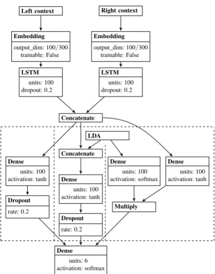
We experiment with three variants of a neural network architecture implemented using Keras6
(Chollet et al., 2015) and visualized in Figure 1.
The word-level representations for the left and right contexts of the emotion word that are re-turned by the embedding layers are fed into
Left context
Embedding output_dim: 100/300
trainable: False
LSTM units: 100 dropout: 0.2
Right context
Embedding output_dim: 100/300
trainable: False
LSTM units: 100 dropout: 0.2
Concatenate
Dense units: 100 activation: tanh
Dropout rate: 0.2
LDA
Concatenate
Dense units: 100 activation: tanh
Dropout rate: 0.2
Dense units: 100 activation: softmax
Dense units: 100 activation: tanh
Multiply
[image:3.595.73.291.57.334.2]Dense units: 6 activation: softmax
Figure 1: Architecture of the three model variants
two unidirectional LSTM layers (Hochreiter and Schmidhuber,1997;Gers et al.,2000): A left-to-right layer for the left context from the beginning of the tweet to the masked emotion word, and a right-to-left layer for the right context from the end of the tweet to the masked emotion word. The hidden states of the two LSTM layers are concate-nated. Now, we explore three variants of incorpo-rating the 100-dimensional LDA topic distribution into the model:
1. We do not use LDA topics. The output of the LSTMs is fed to a dense layer, followed by a dropout layer and finally a softmax output layer.
2. We use LDA topics as features alongside the LSTM output. The LDA topic distribution and the output of the LSTMs are concate-nated. The result is fed to a dense layer, fol-lowed by a dropout layer and finally a soft-max output layer.
3. We use LDA topics as filter. The output of the LSTMs is fed to a dense layer to reduce dimensionality. The LDA topic distribution is fed to a softmax layer. The output of the two layers is combined using element-wise multiplication. The result is fed to the final softmax output layer.
model trial test
train-skip100-nolda 64.06 65.14
train-skip100-ldafeat 64.46 65.10
train-skip100-ldafilt 64.56 65.03
train-skip300-nolda 65.93 66.33
train-skip300-ldafeat 66.05 66.35
train-skip300-ldafilt 65.18 65.79
add-skip100-nolda 52.01 52.12
add-skip100-ldafeat 52.49 52.84
add-skip100-ldafilt 51.29 51.88
add-skip300-nolda 55.28 55.49
add-skip300-ldafeat 55.22 55.11
add-skip300-ldafilt 52.76 52.68
add+train-skip100-nolda 65.19 66.55
add+train-skip100-ldafeat 65.71 66.02 add+train-skip100-ldafilt 65.67 65.94
add+train-skip300-nolda 67.05 67.50
add+train-skip300-ldafeat 67.17 67.08 add+train-skip300-ldafilt 66.43 67.00 add+train+trial-skip300-ldafeat (subm.) 67.13
Table 1: Results for models using skip-gram-based em-beddings (macroF1)
We train each model for a maximum of 20 epochs with a batch size of 160, using the Adam optimizer (Kingma and Ba,2014) to minimize cat-egorical crossentropy. If the validation loss (deter-mined on the trial data) fails to improve for two consecutive epochs, training stops early.
4 Results and Error Analysis 4.1 Experiments
We have three different network architectures that differ in the way they use LDA topic distributions. We have four sets of embeddings that differ in size and training objective. And we have three options for the training data (only the official training data, only our additional data, or training on the latter and retraining on the former). In order to quantify the impact of the individual choices, we train and evaluate all 36 possible models. Results for mod-els using skip-gram-based embeddings are shown in Table 1 and results for models using CBOW-based embeddings in Table2. The evaluation met-ric used is the macro average of the F1 scores of
the six classes.
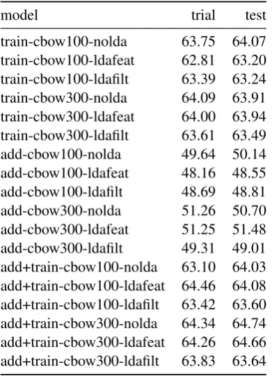
[image:3.595.311.522.68.350.2]model trial test
train-cbow100-nolda 63.75 64.07
train-cbow100-ldafeat 62.81 63.20
train-cbow100-ldafilt 63.39 63.24
train-cbow300-nolda 64.09 63.91
train-cbow300-ldafeat 64.00 63.94
train-cbow300-ldafilt 63.61 63.49
add-cbow100-nolda 49.64 50.14
add-cbow100-ldafeat 48.16 48.55
add-cbow100-ldafilt 48.69 48.81
add-cbow300-nolda 51.26 50.70
add-cbow300-ldafeat 51.25 51.48
add-cbow300-ldafilt 49.31 49.01
[image:4.595.85.281.62.333.2]add+train-cbow100-nolda 63.10 64.03 add+train-cbow100-ldafeat 64.46 64.08 add+train-cbow100-ldafilt 63.42 63.60 add+train-cbow300-nolda 64.34 64.74 add+train-cbow300-ldafeat 64.26 64.66 add+train-cbow300-ldafilt 63.83 63.64
Table 2: Results for models using CBOW-based word embeddings (macroF1)
to differences in the initialization of the weights and the shuffling of the training data.7 However,
since all the individual options have been used at least nine times, we can still make some fairly re-liable claims about their usefulness.
The most obvious observation is that the offi-cial training data lead to much better results than our additional data (+12.97 on average). This is probably due to two reasons: We only use a subset of the emotion words that have been used in the official data sets and, more importantly, we use all instances of the emotion words and not only those that are followed by something that is likely to be a description of the cause of the emotion. How-ever, first training the model on the additional data and then retraining it on the official training data is benefitial (+1.96).
We can also see that word embeddings based on the skip-gram approach consistently outper-form those based on the CBOW approach (+2.55). 300-dimensional embeddings are notably better than 100-dimensional embeddings (+1.19), an ef-fect that is more pronounced for the skip-gram-based embeddings (+1.57) than for the CBOW-based ones (+0.80).
7The 95%-confidence interval for the performance of the
add+train-skip300-ldafeat model on the test data is 67.12±
0.34, for example (estimated from 20 instances of the model).
The LDA topic distributions only have a posi-tive effect when used as additional features along-side the LSTM output – and even then the effect is small and only positive for models using skip-gram-based embeddings (+0.08) and negative for models using CBOW-based embeddings (−0.24).
Using the LDA topic distribution as a filter usually has a negative effect (−0.76).
Consequently, for our submission to the shared task, we chose the second network architecture (LDA topic distribution as feature), used 300-dimensional skip-gram embeddings and trained the model first on our additional data and retrained it on the official training and trial data. That model achieved a macro averageF1score of 67.13 on the
test data and took the tenth place in the shared task. For comparison,Klinger et al. (2018) report that human performance on this task is approximately 45%, the MaxEnt uni- and bigram classifier used as a baseline system achieved 59.88% and the best submission (Rozental et al.,2018) 71.45%. 4.2 Error Analysis
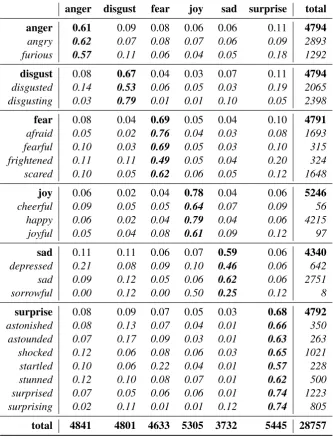
We present detailed error analyses in Table 3 in form of an extensive confusion matrix including label confusion per triggerword in the test data. We downloaded all available tweets used in the shared task via the Twitter API8 to gain access
to the actual triggerwords. For reasons of inter-pretability we report absolute marginal frequen-cies and relative frequenfrequen-cies of predicted label per real label and triggerword.9 This corresponds to
recall (true-positive-rate) for those cases where the prediction equals the true label and false-negative-rate (FNR) per class for all other cases.
Recall is rather similar across labels: The high-est rate can be achieved forjoy(78%), the lowest
is achieved for sad (59%). High FNRs have to
be reported for confusinganger,disgust, andfear
withsurprise(11% and 10%), as well assadwith angeranddisgust(each 11%).
Looking at the recall values per triggerword, ex-planations for the macro-values are not far to seek: 1. Performance is generally higher for those triggerwords that have been manually se-8https://developer.twitter.com/en/docs/
tweets/post-and-engage/api-reference/ get-statuses-lookup
9The difference in absolute numbers between label-based
anger disgust fear joy sad surprise total anger 0.61 0.09 0.08 0.06 0.06 0.11 4794
angry 0.62 0.07 0.08 0.07 0.06 0.09 2893
furious 0.57 0.11 0.06 0.04 0.05 0.18 1292 disgust 0.08 0.67 0.04 0.03 0.07 0.11 4794 disgusted 0.14 0.53 0.06 0.05 0.03 0.19 2065 disgusting 0.03 0.79 0.01 0.01 0.10 0.05 2398
fear 0.08 0.04 0.69 0.05 0.04 0.10 4791 afraid 0.05 0.02 0.76 0.04 0.03 0.08 1693 fearful 0.10 0.03 0.69 0.05 0.03 0.10 315 frightened 0.11 0.11 0.49 0.05 0.04 0.20 324 scared 0.10 0.05 0.62 0.06 0.05 0.12 1648 joy 0.06 0.02 0.04 0.78 0.04 0.06 5246
cheerful 0.09 0.05 0.05 0.64 0.07 0.09 56
happy 0.06 0.02 0.04 0.79 0.04 0.06 4215
joyful 0.05 0.04 0.08 0.61 0.09 0.12 97
sad 0.11 0.11 0.06 0.07 0.59 0.06 4340 depressed 0.21 0.08 0.09 0.10 0.46 0.06 642
sad 0.09 0.12 0.05 0.06 0.62 0.06 2751
sorrowful 0.00 0.12 0.00 0.50 0.25 0.12 8
surprise 0.08 0.09 0.07 0.05 0.03 0.68 4792 astonished 0.08 0.13 0.07 0.04 0.01 0.66 350 astounded 0.07 0.17 0.09 0.03 0.01 0.63 263 shocked 0.12 0.06 0.08 0.06 0.03 0.65 1021 startled 0.10 0.06 0.22 0.04 0.01 0.57 228
stunned 0.12 0.10 0.08 0.07 0.01 0.62 500
surprised 0.07 0.05 0.06 0.06 0.01 0.74 1223 surprising 0.02 0.11 0.01 0.01 0.12 0.74 805
[image:5.595.132.466.64.504.2]total 4841 4801 4633 5305 3732 5445 28757
Table 3: Confusion Matrix for the six predicted emotion categories (columns) for each real emotion and each triggerword (rows) in the test data
lected by us for producing additional training data (see Section 3.3): angry (62%) shows
higher recall than furious (57%), afraid
(76%) andhappy(79%) perform best in the fearandjoycategories, respectively, and sur-prisedandsurprising(each 74%) are the best
predictors forsurprise.
2. Rare triggerwords generally lead to worse re-sults. The most obvious example is sorrow-ful, which we only observed 28 times in the
training data (8 times in the test data) and which yields 25% recall for predicting cate-gorysad, confusing it in half of the cases with joy. Additionally, cheerful and joyful (361
and 536 observations in the training data,
re-spectively) perform lower thanhappy(22348
observations) – although admittedly happy
had already been pre-selected for additional training as mentioned above.
3. Many confusions can also be explained from a psycho-linguistic point of view when look-ing at the actual corpus. Instances involvlook-ing the triggerworddisgustede. g. are frequently
categorized asanger by our system. Corpus
evidence shows that these words are hard to disambiguate:
• Hindu women should be
model trial test
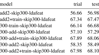
add2-skip300-ldafeat 56.66 56.98
add2+train-skip300-ldafeat 67.34 67.47 300-train-skip300-ldafeat 66.14 66.68
300-add-skip300-ldafeat 57.10 57.29
300-add+train-skip300-ldafeat 67.89 68.06
300-add2-skip300-ldafeat 58.35 58.49
300-add2+train-skip300-ldafeat 67.98 68.10
Table 4: Results for the post-analysis experiments (macroF1)
women are property of Father-In-Law?
• I wake up [#TRIGGERWORD#]
be-cause I know you doin me wrong but u dont think its nothing wrong with being in a verbal relationship with another gal
It is hard to see how one could reliably pre-dict the “real” emotion (disgust) in the above
examples, sinceanger– as predicted by our
system – seems to be an equally sensible guess. Similar instances can be found for other confusions, most notably when pre-dicting anger in case of the triggerword de-pressed.
4.3 Post-analysis experiments
The analysis in the previous section has shown that our system performs better on the more frequent words that we used for compiling our additional data than on the less frequent words. Therefore, we recompile our additional data as described in Section 3.3 but for all of the 21 emotion words that occur in the official data. After balancing the data, this results in approximately 163.000 items per class.
We take the model versions from Section 4.1 that are the basis for our submission and replace the additional data with the updated version. The new models (prefixed with “add2” in Table4) im-prove on the old ones both when using only the additional data (+1.66) and when retraining on the official training data (+0.28).
It is also worth pointing out that so far we have not fine-tuned the hyperparameters of our model. As a first step in that direction, we try to use more units in the hidden layers and increase the size of all hidden layers to 300 units (models prefixed with “300-add” in Table 4). This boosts the per-formance both when using only the additional data
(+2.03) and when retraining on the official training data (+0.85).
Combining the recompiled additional data and the larger hidden layers yields further improve-ments (models prefixed with “300-add2” in Ta-ble 4). The retrained model is approximately 1 point better than our submission and would have taken the eighth place in the shared task.
A further error analysis shows that the addi-tional training data indeed yield the desired effect: Recall for categoryangryimproves from 61% to
66%, largely due to better recall in the case of the triggerwordfurious(rising from 57% to 65%).
Further improvements can be found in almost all categories, namely for fear (69% to 72%,
espe-ciallyfrightened: 49% to 53%),joy(78% to 79%,
with recall forjoyfulrising from 61% to 65% and
forcheerful from 64% to 70%), andsad(59% to
62%, triggerword depressed up two points from
46% to 48%). However, the additional training data had an adverse effect on category surprise;
here recall falls from 68% to 65%, with almost all triggerwords dropping a couple of points, the worst beingsurprised, falling from 74% to 69%.
Finally, we want to take a closer look at the contribution of the LDA topic distribution. To this end, we have trained 20 instances of the skip300-ldafeat and 300-add2+train-skip300-nolda models and have calculated the means and 95%-confidence intervals. As it turns out, both model variants perform identically on the trial data. On the test data, there are some minor differences but the performance means lie within one standard deviation of each other. This means that our choice of concatenating the LDA topic distribution of the tweet to the LSTM does not have a statistically significant result..
5 Conclusion
We presented EmotiKLUE, a topic-informed deep learning system for detecting implicit emo-tion. Our experiments showed that for this task skip-gram-based word embeddings outper-form CBOW-based embeddings. Additional data, that – on their own – yield rather poor results, im-prove the performance when used for pretraining the model. LDA topic models, that we initially be-lieved to have a small positive effect, turned out to not contribute significantly.
[image:6.595.76.287.64.182.2]many instances of tweets showing prima facie am-biguous emotions, it is unsurprising that even per-fectly trained classifiers will not be able to achieve 100% accuracy when using the textual data alone. Future work could nonetheless involve more ex-perimentation with the hyperparameters of the net-work, e. g. number, size and activation of the hid-den layers, choice of regularization strategy and optimizer, etc.
The software is available on GitHub.10
References
David M. Blei, Andrew Y. Ng, and Michael I. Jordan. 2003. Latent dirichlet allocation. Journal of Ma-chine Learning Research, 3:993–1022.
Franc¸ois Chollet et al. 2015. Keras. https://keras. io.
Stefan Evert, Thomas Proisl, Paul Greiner, and Besim Kabashi. 2014. SentiKLUE: Updating a polarity classifier in 48 hours. InProceedings of the 8th In-ternational Workshop on Semantic Evaluation (Se-mEval 2014), pages 551–555, Dublin. Association for Computational Linguistics.
Syeda Nadia Firdaus, Chen Ding, and Alireza Sadeghian. 2018. Topic specific emotion detection for retweet prediction.International Journal of Ma-chine Learning and Cybernetics, pages 197–203. Felix A. Gers, J¨urgen Schmidhuber, and Fred A.
Cummins. 2000. Learning to forget: Contin-ual prediction with LSTM. Neural Computation, 12(10):2451–2471.
Diman Ghazi, Diana Inkpen, and Stan Szpakowicz. 2015.Detecting emotion stimuli in emotion-bearing sentences. InComputational Linguistics and Intel-ligent Text Processing. CICLing 2015, pages 152– 165.
Sepp Hochreiter and J¨urgen Schmidhuber. 1997.
Long short-term memory. Neural Computation, 9(8):1735–1780.
Diederik P. Kingma and Jimmy Ba. 2014. Adam: A method for stochastic optimization. CoRR, abs/1412.6980.
Roman Klinger, Orph´ee de Clercq, Saif M. Moham-mad, and Alexandra Balahur. 2018. IEST: WASSA-2018 Implicit Emotions Shared Task. In Proceed-ings of the 9th Workshop on Computational Ap-proaches to Subjectivity, Sentiment and Social Me-dia Analysis, Brussels. ACL.
Sophia Yat Mei Lee. 2015.A linguistic analysis of im-plicit emotions. InChinese Lexical Semantics - 16th Workshop, CLSW 2015, Beijing, China, May 9-11, 2015, Revised Selected Papers, pages 185–194.
10https://github.com/tsproisl/EmotiKLUE
Tomas Mikolov, Kai Chen, Greg Corrado, and Jeffrey Dean. 2013a. Efficient estimation of word represen-tations in vector space.CoRR, abs/1301.3781.
Tomas Mikolov, Ilya Sutskever, Kai Chen, Gregory S. Corrado, and Jeffrey Dean. 2013b. Distributed rep-resentations of words and phrases and their com-positionality. In Advances in Neural Information Processing Systems 26: 27th Annual Conference on Neural Information Processing Systems 2013. Pro-ceedings of a meeting held December 5-8, 2013, Lake Tahoe, Nevada, United States., pages 3111– 3119.
Saif M. Mohammad, Parinaz Sobhani, and Svetlana Kiritchenko. 2017. Stance and sentiment in tweets. Special Section of the ACM Transactions on Inter-net Technology on Argumentation in Social Media, 17(3).
A. Ortony, G. Clore, and A. Collins. 1988. Cognitive Structure of Emotions. Cambridge University Press.
Thomas Proisl, Paul Greiner, Stefan Evert, and Besim Kabashi. 2013. KLUE: Simple and robust meth-ods for polarity classification. InProceedings of the 7th International Workshop on Semantic Evaluation (SemEval 2013), pages 395–401, Atlanta, GA. As-sociation for Computational Linguistics.
Thomas Proisl and Peter Uhrig. 2016. SoMaJo: State-of-the-art tokenization for German web and social media texts. InProceedings of the 10th Web as Cor-pus Workshop (WAC-X) and the EmpiriST Shared Task, pages 57–62, Berlin. ACL.
Han Ren, Yafeng Ren, Xia Li, Wenhe Feng, and Maofu Liu. 2017. Natural logic inference for emotion de-tection. In Proceedings of CCL 2017 and NLP-NABD 2017, pages 424–436.
Jitendra Kumar Rout, Kim-Kwang Raymond Choo, Amiya Kumar Dash, Sambit Bakshi, Sanjay Ku-mar Jena, and Karen L. Williams. 2018. A model for sentiment and emotion analysis of unstructured social media text. Electronic Commerce Research, 18(1):181–199.
Alon Rozental, Daniel Fleischer, and Zohar Kelrich. 2018. Amobee at IEST 2018: Transfer learning from language models. In Proceedings of the 9th Workshop on Computational Approaches to Subjec-tivity, Sentiment and Social Media Analysis, Brus-sels. ACL.
Kashfia Sailunaz, Manmeet Dhaliwal, Jon Rokne, and Reda Alhajj. 2018. Emotion detection from text and speech: a survey.Social Network Analysis and Min-ing, 8(1):28:1–28:26.
Klaus R. Scherer. 2005. What are emotions? And how can they be measured? Social Science Information, 44(4):695–729.
Fabian Sch¨afer, Stefan Evert, and Philipp Heinrich. 2017. Japan’s 2014 General Election: Political Bots, Right-Wing Internet Activism and PM Abe Shinz¯o’s Hidden Nationalist Agenda. Big Data, 5(4):294– 309.
Roland Sch¨afer. 2015. Processing and querying large web corpora with the COW14 architecture. In Proceedings of Challenges in the Management of Large Corpora 3 (CMLC-3), pages 28–34, Lan-caster. UCREL, IDS.
Roland Sch¨afer and Felix Bildhauer. 2012. Building large corpora from the web using a new efficient tool chain. InProceedings of the Eighth International Conference on Language Resources and Evaluation (LREC 2012), pages 486–493, Istanbul. ELRA.
Orizu Udochukwu and Yulan He. 2015. A rule-based approach to implicit emotion detection in text. In Proceedings of NLDB 2015, pages 197–203.