Proceedings of the 9th Workshop on Computational Approaches to Subjectivity, Sentiment and Social Media Analysis, pages 50–56 Brussels, Belgium, October 31, 2018. c2018 Association for Computational Linguistics
50
IIIDYT at IEST 2018: Implicit Emotion Classification With Deep
Contextualized Word Representations
Jorge A. Balazs, Edison Marrese-Taylor and Yutaka Matsuo
Graduate School of Engineering The University of Tokyo
{jorge, emarrese, matsuo}@weblab.t.u-tokyo.ac.jp
Abstract
In this paper we describe our system designed for the WASSA 2018 Implicit Emotion Shared Task (IEST), which obtained 2nd place out
of 30 teams with a test macro F1 score of
0.710. The system is composed of a single pre-trained ELMo layer for encoding words, a Bidirectional Long-Short Memory Network BiLSTM for enriching word representations with context, a max-pooling operation for cre-ating sentence representations from them, and a Dense Layer for projecting the sentence representations into label space. Our offi-cial submission was obtained by ensembling 6 of these models initialized with different ran-dom seeds. The code for replicating this pa-per is available athttps://github.com/ jabalazs/implicit_emotion.
1 Introduction
Although the definition of emotion is still debated among the scientific community, the automatic identification and understanding of human emo-tions by machines has long been of interest in computer science. It has usually been assumed that emotions are triggered by the interpretation of a stimulus event according to its meaning.
As language usually reflects the emotional state of an individual, it is natural to study human emo-tions by understanding how they are reflected in text. We see that many words indeed have af-fect as a core part of their meaning, for example, dejectedandwistfuldenote some amount of sad-ness, and are thus associated with sadness. On the other hand, some words are associated with af-fect even though they do not denote afaf-fect. For example,failureanddeath describe concepts that are usually accompanied by sadness and thus they denote some amount of sadness. In this context, the task of automatically recognizing emotions from text has recently attracted the attention of
re-searchers in Natural Language Processing. This task is usually formalized as the classification of words, phrases, or documents into predefined dis-crete emotion categories or dimensions. Some ap-proaches have aimed at also predicting the degree to which an emotion is expressed in text ( Moham-mad and Bravo-Marquez,2017).
In light of this, the WASSA 2018 Implicit Emo-tion Shared Task (IEST) (Klinger et al., 2018) was proposed to help find ways to automatically learn the link between situations and the emotion they trigger. The task consisted in predicting the emotion of a word excluded from a tweet. Re-moved words, ortrigger-words, included the terms “sad”, “happy”, “disgusted”, “surprised”, “angry”, “afraid” and their synonyms, and the task was to predict the emotion they conveyed, specifically sadness, joy, disgust, surprise, anger and fear.
From a machine learning perspective, this prob-lem can be seen as sentence classification, in which the goal is to classify a sentence, or in par-ticular a tweet, into one of several categories. In the case of IEST, the problem is specially chal-lenging since tweets contain informal language, the heavy usage of emoji, hashtags and username mentions.
our system, which we plan to release, is the first to utilize ELMo for emotion recognition.
2 Proposed Approach
2.1 Preprocessing
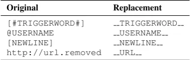
As our model is purely character-based, we per-formed little data preprocessing. Table 1 shows the special tokens found in the datasets, and how we substituted them.
Original Replacement
[image:2.595.84.278.205.266.2][#TRIGGERWORD#] TRIGGERWORD @USERNAME USERNAME [NEWLINE] NEWLINE http://url.removed URL
Table 1: Preprocessing substitutions.
Furthermore, we tokenized the text using a vari-ation of the twokenize.py1 script, a Python port of the originalTwokenize.java(Gimpel et al., 2011). Concretely, we created an emoji-aware version of it by incorporating knowledge from an emoji database,2 which we slightly mod-ified for avoiding conflict with emoji sharing uni-code uni-codes with common glyphs used in Twitter,3 and for making it compatible with Python 3.
2.2 Architecture
Figure 1 summarizes our proposed architecture. Our input is based on Embeddings from Language Models (ELMo) by Peters et al. (2018). These are character-based word representations allowing the model to avoid the “unknown token” problem. ELMo uses a set of convolutional neural networks to extract features from character embeddings, and builds word vectors from them. These are then fed to a multi-layer Bidirectional Language Model (BiLM) which returns context-sensitive vectors for each input word.
We used a single-layer BiLSTM as context fine-tuner (Graves and Schmidhuber, 2005; Graves et al.,2013), on top of the ELMo embeddings, and then aggregated the hidden states it returned by us-ing max-poolus-ing, which has been shown to per-form well on sentence classification tasks ( Con-neau et al.,2017).
1
https://github.com/myleott/ark- twokenize- py
2
https://github.com/carpedm20/emoji/blob/e7bff32/emoji/ unicode_codes.py
3For example, the hashtag emoji is composed by the
uni-code uni-code pointsU+23 U+FE0F U+20E3, which include
U+23, the same code point for the#glyph.
Finally, we used a single-layer fully-connected network for projecting the pooled BiLSTM output into a vector corresponding to the label logits for each predicted class.
2.3 Implementation Details and
Hyperparameters
ELMo Layer: We used the official
Al-lenNLP implementation of the ELMo model4, with the official weights pre-trained on the 1 Bil-lion Word Language Model Benchmark, which contains about 800M tokens of news crawl data from WMT 2011 (Chelba et al.,2014).
Dimensionalities: By default the ELMo layer
outputs a 1024-dimensional vector, which we then feed to a BiLSTM with output size 2048, resulting in a 4096-dimensional vector when concatenating forward and backward directions for each word of the sequence5. After max-pooling the BiLSTM output over the sequence dimension, we obtain a single 4096-dimensional vector corresponding to the tweet representation. This representation is fi-nally fed to a single-layer fully-connected network with input size 4096, 512 hidden units, output size 6, and a ReLU nonlinearity after the hidden layer. The output of the dense layer is a 6-dimensional logit vector for each input example.
Loss Function: As this corresponds to a
mul-ticlass classification problem (predicting a single class for each example, with more than 2 classes to choose from), we used the Cross-Entropy Loss as implemented in PyTorch (Paszke et al.,2017).
Optimization: We optimized the model with
Adam (Kingma and Ba, 2014), using default hy-perparameters (β1 = 0.9,β2 = 0.999,= 10−8), following a slanted triangular learning rate sched-ule (Howard and Ruder,2018), also with default hyperparameters (cut f rac = 0.1, ratio = 32), and a maximum learning rateηmax= 0.001, over T = 23,970iterations6.
Regularization: we used a dropout layer (
Sri-vastava et al., 2014), with probability of 0.5 af-ter both the ELMo and the hidden fully-connected layer, and another one with probability of 0.1
af-4
https://allenai.github.io/allennlp- docs/api/allennlp. modules.elmo.html
5A BiLSTM is composed of two separate LSTMs that read
the input in opposite directions and whose outputs are con-catenated at the hidden dimension. This results in a vector double the dimension of the input for each time step.
6This number is obtained by multiplying the number of
epochs (10), times the total number of batches, which for the
training dataset corresponds to2396batches of64elements,
BiLSTM
ELMo Layer Max Pooling
Context Layer Sentence Encoder
Fully-Connected Network
Softmax
Probabilities
Classifier [#TRIGGERWORD#]
It’s
...
[image:3.595.113.488.61.224.2]Word Encoder
Figure 1: Proposed architecture.
ter the max-pooling aggregation layer. We also reshuffled the training examples between epochs, resulting in a different batch for each iteration.
Model Selection: To choose the best
hyperpa-rameter configuration we measured the classifica-tion accuracy on the validaclassifica-tion (trial) set.
2.4 Ensembles
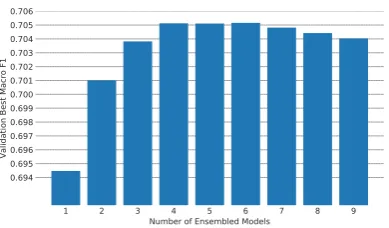
Once we found the best-performing configura-tion we trained 10 models using different random seeds, and tried averaging the output class prob-abilities of all their possible P9
k=1 9 k
= 511 combinations. As Figure 2 shows, we empiri-cally found that a specific combination of6 mod-els yielded the best results (70.52%), providing ev-idence for the fact that using a number of indepen-dent classifiers equal to the number of class labels provides the best results when doing average en-sembling (Bonab and Can,2016).
1 2 3 4 5 6 7 8 9
Number of Ensembled Models 0.694
0.695 0.696 0.697 0.698 0.699 0.700 0.701 0.702 0.703 0.704 0.705 0.706
Va
lid
ati
on
Be
st
Ma
cro
F1
Figure 2: Effect of the number of ensembled mod-els on validation performance.
3 Experiments and Analyses
We performed several experiments to gain insights on how the proposed model’s performance
inter-acts with the shared task’s data. We performed an ablation study to see how some of the main hy-perparameters affect performance, and an analy-sis of tweets containing hashtags and emoji to un-derstand how these two types of tokens help the model predict the trigger-word’s emotion. We also observed the effects of varying the amount of data used for training the model to evaluate whether it would be worthwhile to gather more training data.
3.1 Ablation Study
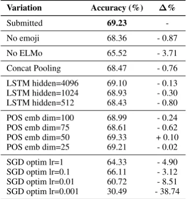
We performed an ablation study on a single model having obtained 69.23% accuracy on the valida-tion set. Results are summarized in Table2.
We can observe that the architectural choice that had the greatest impact on our model was the ELMo layer, providing a3.71%boost in per-formance as compared to using GloVe pre-trained word embeddings.
We can further see that emoji also contributed significantly to the model’s performance. In Sec-tion 3.4 we give some pointers to understanding why this is so.
Additionally, we tried using the concatenation of the max-pooled, average-pooled and last hidden states of the BiLSTM as the sentence represen-tation, following Howard and Ruder (2018), but found out that this impacted performance nega-tively. We hypothesize this is due to tweets be-ing too short for needbe-ing such a rich representa-tion. Also, the size of the concatenated vector was 4096×3 = 12,288, which probably could not be properly exploited by the512-dimensional fully-connected layer.
[image:3.595.76.271.543.657.2]Variation Accuracy (%) ∆%
Submitted 69.23
-No emoji 68.36 - 0.87
No ELMo 65.52 - 3.71
Concat Pooling 68.47 - 0.76
LSTM hidden=4096 69.10 - 0.13
LSTM hidden=1024 68.93 - 0.30
LSTM hidden=512 68.43 - 0.80
POS emb dim=100 68.99 - 0.24
POS emb dim=75 68.61 - 0.62
POS emb dim=50 69.33 + 0.10
POS emb dim=25 69.21 - 0.02
SGD optim lr=1 64.33 - 4.90
SGD optim lr=0.1 66.11 - 3.12
SGD optim lr=0.01 60.72 - 8.51
[image:4.595.304.527.61.241.2]SGD optim lr=0.001 30.49 - 38.74
Table 2: Ablation study results.
Accuracies were obtained from the validation dataset. Each model was trained with the same random seed and hyperpa-rameters, save for the one listed. “No emoji” is the same model trained on the training dataset with no emoji, “No ELMo” corresponds to having switched the ELMo word en-coding layer with a simple pre-trained GloVe embedding lookup table, and “Concat Pooling” obtained sentence
repre-sentations by using the pooling method described byHoward
and Ruder(2018). “LSTM hidden” corresponds to the hidden
dimension of the BiLSTM, “POS emb dim” to the dimen-sion of the part-of-speech embeddings, and “SGD optim lr” to the learning rate used while optimizing with the schedule
described byConneau et al.(2017).
mentioned earlier; the fully-connected layer was not big or deep enough to exploit the additional in-formation. Similarly, using a smaller hidden size neither helped.
We found that using 50-dimensional part-of-speech embeddings slightly improved results, which implies that better fine-tuning this hyperpa-rameter, or using a better POS tagger could yield an even better performance.
Regarding optimization strategies, we also tried using SGD with different learning rates and a step-wise learning rate schedule as described by Con-neau et al.(2018), but we found that doing this did not improve performance.
Finally, Figure 3shows the effect of using dif-ferent dropout probabilities. We can see that hav-ing higher dropout after the word-representation layer and the fully-connected network’s hidden layer, while having a low dropout after the sen-tence encoding layer yielded better results overall.
3.2 Error Analysis
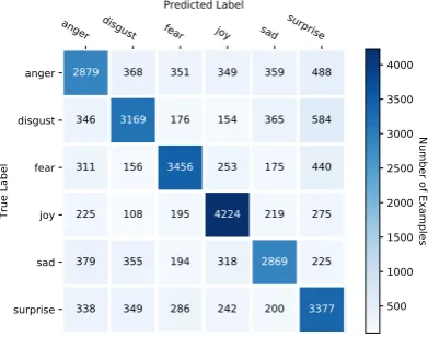
Figure 4 shows the confusion matrix of a single model evaluated on the test set, and Table 3 the
0.0 Dropout after sentence-encoding layer0.1 0.2 0.3 0.4 0.5 0.6
0.0
0.1
0.2
0.3
0.4
0.5
0.6
Dropout after word-encoding & fully-connected layers
67.92 67.52 68.12 67.77 68.04 67.43 67.71
67.94 67.66 68.17 68.21 67.89 67.72 67.73
67.86 68.54 68.66 68.10 68.07 68.18 67.68
68.43 68.23 68.32 68.33 68.51 68.30 68.07
68.80 68.91 68.66 68.71 68.46 68.48 68.19
68.82 69.23 68.99 68.95 68.49 69.04 68.53
68.96 68.86 68.50 68.92 68.61 68.56 68.17 67.6
67.8 68.0 68.2 68.4 68.6 68.8 69.0 69.2
Validation Accuracy (%)
Figure 3: Dropout Ablation.
Rows correspond to the dropout applied both after the ELMo layer (word encoding layer) and after the fully-connected net-work’s hidden layer, while columns correspond to the dropout applied after the max-pooling operation (sentence encoding layer.)
corresponding classification report. In general, we confirm whatKlinger et al.(2018) report:anger was the most difficult class to predict, followed by surprise, whereasjoy,fear, anddisgust are the better performing ones.
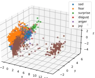
To observe whether any particular pattern arose from the sentence representations encoded by our model, we projected them into 3d space through Principal Component Analysis (PCA), and were surprised to find that 2 clearly defined clus-ters emerged (see Figure 6), one containing the majority of datapoints, and another containing joy tweets exclusively. Upon further explo-ration we also found that the smaller cluster was composed only by tweets containing the pattern un TRIGGERWORD , and further, that all of them were correctly classified.
It is also worth mentioning that there are 5827 tweets in the training set with this pat-tern. Of these, 5822 (99.9%) correspond to the label joy. We observe a similar trend on the test set; 1115 of the 1116 tweets having theun TRIGGERWORD pattern correspond to joytweets. We hypothesize this is the reason why the model learned this pattern as a strong discrim-inating feature.
Finally, the only tweet in the test set that con-tained this pattern and did not belong to thejoy class, originally had unsurprised as its trigger-word7, and unsurprisingly, was misclassified.
[image:4.595.86.277.63.266.2]anger disgust fearPredicted Labeljoy sad surprise
anger
disgust
fear
joy
sad
surprise
True Label
2879 368 351 349 359 488
346 3169 176 154 365 584
311 156 3456 253 175 440
225 108 195 4224 219 275
379 355 194 318 2869 225
338 349 286 242 200 3377 500 1000 1500 2000 2500 3000 3500 4000
[image:5.595.327.503.64.104.2]Number of Examples
Figure 4: Confusion Matrix (Test Set).
Precision Recall F1-score
anger 0.643 0.601 0.621
disgust 0.703 0.661 0.682
fear 0.742 0.721 0.732
joy 0.762 0.805 0.783
sad 0.685 0.661 0.673
surprise 0.627 0.705 0.663
[image:5.595.87.283.68.222.2]Average 0.695 0.695 0.694
Table 3: Classification Report (Test Set).
3.3 Effect of the Amount of Training Data
As Figure5shows, increasing the amount of data with which our model was trained consistently in-creased validation accuracy and validation macro F1 score. The trend suggests that the proposed model is expressive enough to learn from more data, and is not overfitting the training set.
0.2 0.4 0.6 0.8 1.0 Training Data Proportion
0.63 0.64 0.65 0.66 0.67 0.68 0.69 0.70
V
al
id
at
io
n
Sc
or
e
Best Validation Accuracy
Best Validation Average Macro F1 Score
Figure 5: Effect of the amount of training data on classification performance.
3.4 Effect of Emoji and Hashtags
Table 4 shows the overall effect of hashtags and emoji on classification performance. Tweets
con-Present Not Present
Emoji 4805 (76.6%) 23952 (68.0%)
Hashtags 2122 (70.5%) 26635 (69.4%)
Table 4: Number of tweets on the test set with and without emoji and hashtags. The number between parentheses is the proportion of tweets classified correctly.
taining emoji seem to be easier for the model to classify than those without. Hashtags also have a positive effect on classification performance, how-ever it is less significant. This implies that emoji, and hashtags in a smaller degree, provide tweets with a context richer in sentiment information, al-lowing the model to better guess the emotion of thetrigger-word.
Emoji alias N emoji no-emoji ∆%
# % # %
[image:5.595.90.273.263.360.2] [image:5.595.307.526.330.468.2]mask 163 154 94.48 134 82.21 - 12.27 two hearts 87 81 93.10 77 88.51 - 4.59 heart eyes 122 109 89.34 103 84.43 - 4.91 heart 267 237 88.76 235 88.01 - 0.75 rage 92 78 84.78 66 71.74 - 13.04 cry 116 97 83.62 83 71.55 - 12.07 sob 490 363 74.08 345 70.41 - 3.67 unamused 167 121 72.46 116 69.46 - 3.00 weary 204 140 68.63 139 68.14 - 0.49 joy 978 649 66.36 629 64.31 - 2.05 sweat smile 111 73 65.77 75 67.57 1.80 confused 77 46 59.74 48 62.34 2.60
Table 5: Fine grained performance on tweets con-taining emoji, and the effect of removing them.
Nis the total number of tweets containing the listed emoji,
#and%the number and percentage of correctly-classified
tweets respectively, and∆%the variation of test accuracy
when removing the emoji from the tweets.
Table 5 shows the effect specific emoji have on classification performance. It is clear some emoji strongly contribute to improving prediction quality. The most interesting ones are mask, rage, and cry, which significantly increase ac-curacy. Further, contrary to intuition, the sob emoji contributes less thancry, despite represent-ing a stronger emotion. This is probably due to sobbeing used for depicting a wider spectrum of emotions.
Finally, not all emoji are beneficial for this task.
When removingsweat smileandconfused
[image:5.595.75.270.529.659.2]x 2 0 2 4
6 8 10 1214 20 y 2 4
6 z
[image:6.595.119.272.82.207.2]4 2 0 2 4 6 sad fear surprise disgust anger joy
Figure 6: 3d Projection of the Test Sentence Rep-resentations.
4 Conclusions and Future Work
We described the model that got second place in the WASSA 2018 Implicit Emotion Shared Task. Despite its simplicity, and low amount of depen-dencies on libraries and external features, it per-formed almost as well as the system that obtained the first place.
Our ablation study revealed that our hyperpa-rameters were indeed quite well-tuned for the task, which agrees with the good results obtained in the official submission. However, the ablation study also showed that increased performance can be ob-tained by incorporating POS embeddings as addi-tional inputs. Further experiments are required to accurately measure the impact that this additional input may have on the results. We also think the performance can be boosted by making the archi-tecture more complex, concretely, by using a BiL-STM with multiple layers and skip connections in a way akin to (Peters et al., 2018), or by making the fully-connected network bigger and deeper.
We also showed that, what was probably an annotation artifact, the un TRIGGERWORD pattern, resulted in increased performance for the joy label. This pattern was probably originated by a heuristic na¨ıvely replacing the ocurrence of happy by the trigger-word indica-tor. We think the dataset could be improved by replacing the word unhappy, in the
origi-nal examples, by TRIGGERWORD instead of
un TRIGGERWORD , and labeling it as sad, orangry, instead ofjoy.
Finally, our studies regarding the importance of hashtags and emoji in the classification showed that both of them seem to contribute significantly
to the performance, although in different mea-sures.
5 Acknowledgements
We thank the anonymous reviewers for their re-views and suggestions. The first author is partially supported by the Japanese Government MEXT Scholarship.
References
Hamed R. Bonab and Fazli Can. 2016. A theoretical framework on the ideal number of classifiers for on-line ensembles in data streams. InProceedings of the 25th ACM International on Conference on In-formation and Knowledge Management, CIKM ’16, pages 2053–2056, New York, NY, USA. ACM.
Ciprian Chelba, Tomas Mikolov, Mike Schuster, Qi Ge, Thorsten Brants, Phillipp Koehn, and Tony Robin-son. 2014. One billion word benchmark for measur-ing progress in statistical language modelmeasur-ing. Pro-ceedings of the Annual Conference of the Interna-tional Speech Communication Association, INTER-SPEECH, pages 2635–2639.
Alexis Conneau, Douwe Kiela, Holger Schwenk, Lo¨ıc Barrault, and Antoine Bordes. 2017. Supervised Learning of Universal Sentence Representations from Natural Language Inference Data. In Proceed-ings of the 2017 Conference on Empirical Methods in Natural Language Processing, pages 670–680, Copenhagen, Denmark. Association for Computa-tional Linguistics.
Alexis Conneau, Germ´an Kruszewski, Guillaume Lample, Lo¨ıc Barrault, and Marco Baroni. 2018. What you can cram into a single vector: Probing sentence embeddings for linguistic properties. In
Proceedings of the 56th Annual Meeting of the As-sociation for Computational Linguistics (Volume 1: Long Papers), pages 2126–2136. Association for Computational Linguistics.
Kevin Gimpel, Nathan Schneider, Brendan O’Connor, Dipanjan Das, Daniel Mills, Jacob Eisenstein, Michael Heilman, Dani Yogatama, Jeffrey Flani-gan, and Noah A. Smith. 2011. Part-of-speech tag-ging for twitter: Annotation, features, and experi-ments. In Proceedings of the 49th Annual Meet-ing of the Association for Computational LMeet-inguis- Linguis-tics: Human Language Technologies, pages 42–47, Portland, Oregon, USA. Association for Computa-tional Linguistics.
Alex Graves and J¨urgen Schmidhuber. 2005. Frame-wise Phoneme Classification with Bidirectional LSTM and Other Neural Network Architectures.
Neural Networks, 18(5-6):602–610.
Jeremy Howard and Sebastian Ruder. 2018. Universal Language Model Fine-tuning for Text Classification.
ArXiv e-prints.
Diederik P. Kingma and Jimmy Ba. 2014. Adam: A method for stochastic optimization.CoRR.
Roman Klinger, Orph´ee de Clercq, Saif M. Moham-mad, and Alexandra Balahur. 2018. IEST: WASSA-2018 Implicit Emotions Shared Task. In Proceed-ings of the 9th Workshop on Computational Ap-proaches to Subjectivity, Sentiment and Social Me-dia Analysis, Brussels, Belgium. Association for Computational Linguistics.
Saif M. Mohammad and Felipe Bravo-Marquez. 2017. WASSA-2017 Shared Task on Emotion Intensity. In
Proceedings of the EMNLP 2017 Workshop on Com-putational Approaches to Subjectivity, Sentiment, and Social Media (WASSA), Copenhagen, Denmark.
Adam Paszke, Sam Gross, Soumith Chintala, Gre-gory Chanan, Edward Yang, Zachary DeVito, Zem-ing Lin, Alban Desmaison, Luca Antiga, and Adam Lerer. 2017. Automatic differentiation in pytorch. InNIPS Autodiff Workshop.
Matthew Peters, Mark Neumann, Mohit Iyyer, Matt Gardner, Christopher Clark, Kenton Lee, and Luke Zettlemoyer. 2018. Deep contextualized word rep-resentations. In Proceedings of the 2018 Confer-ence of the North American Chapter of the Associ-ation for ComputAssoci-ational Linguistics: Human Lan-guage Technologies, Volume 1 (Long Papers), pages 2227–2237, New Orleans, Louisiana. Association for Computational Linguistics.