A Bayesian mixture model for term re-occurrence and burstiness
Avik Sarkar1, Paul H Garthwaite2, Anne De Roeck1 1Department of Computing,2 Department of Statistics
The Open University Milton Keynes, MK7 6AA, UK
{a.sarkar, p.h.garthwaite, a.deroeck}@open.ac.uk
Abstract
This paper proposes a model for term re-occurrence in a text collection based on the gaps between successive occurrences of a term. These gaps are modeled using a mixture of exponential distributions. Pa-rameter estimation is based on a Bayesian framework that allows us to fit a flexi-ble model. The model provides measures of a term’s re-occurrence rate and
within-document burstiness. The model works
for all kinds of terms, be it rare content word, medium frequency term or frequent function word. A measure is proposed to account for the term’s importance based on its distribution pattern in the corpus.
1 Introduction
Traditionally, Information Retrieval(IR)and Statis-tical Natural Language Processing (NLP) applica-tions have been based on the “bag of words” model. This model assumes term independence and homo-geneity of the text and document under considera-tion, i.e. the terms in a document are all assumed to be distributed homogeneously. This immediately leads to the Vector Space representation of text. The immense popularity of this model is due to the ease with which mathematical and statistical techniques can be applied to it.
The model assumes that once a term occurs in a document, its overall frequency in the entire doc-ument is the only useful measure that associates a
term with a document. It does not take into consid-eration whether the term occurred in the beginning, middle or end of the document. Neither does it con-sider whether the term occurs many times in close succession or whether it occurs uniformly through-out the document. It also assumes that additional positional information does not provide any extra leverage to the performance of the NLP and IR ap-plications based on it. This assumption has been shown to be wrong in certain applications (Franz, 1997).
Existing models for term distribution are based on the above assumption, so they can merely estimate the term’s frequency in a document or a term’s top-ical behavior for a content term. The occurrence of a content word is classified as topical or non-topical based on whether it occurs once or many times in the document (Katz, 1996). We are not aware of any existing model that makes less stringent assumptions and models the distribution of occurrences of a term. In this paper we describe a model for term re-occurrence in text based on the gaps between succes-sive occurrences of the term and the position of its first occurrence in a document. The gaps are mod-eled by a mixture of exponential distributions. Non-occurrence of a term in a document is modeled by the statistical concept of censoring, which states that the event of observing a certain term is censored at the end of the document, i.e. the document length. The modeling is done in a Bayesian framework.
The organization of the paper is as follows. In section 2 we discuss existing term distribution mod-els, the issue of burstiness and some other work that demonstrates the failure of the “bag of words”
sumption. In section 3 we describe our mixture model, the issue of censoring and the Bayesian for-mulation of the model. Section 4 describes the Bayesian estimation theory and methodology. In section 5 we talk about ways of drawing infer-ences from our model, present parameter estimates on some chosen terms and present case studies for a few selected terms. We discuss our conclusions and suggest directions for future work in section 6.
2 Existing Work
2.1 Models
Previous attempts to model a term’s distribution pat-tern have been based on the Poisson distribution. If the number of occurrences of a term in a document is denoted byk, then the model assumes:
p(k) = e−λλ
k
k!
for k = 0,1,2, . . . Estimates based on this model are good for non-content, non-informative terms, but not for the more informative content terms (Manning and Sch¨utze, 1999).
The two-Poisson model is suggested as a variation of the Poisson distribution (Bookstein and Swanson, 1974; Church and Gale, 1995b). This model sumes that there are two classes of documents as-sociated with a term, one class with a low average number of occurrences and the other with a high av-erage number of occurrences.
p(k) = αe−λ1λk1
k! + (1−α)e
−λ2λk2
k!,
where α and (1−α) denote the probabilities of a document in each of these classes. Often this model under-estimates the probability that a term will oc-cur exactly twice in a document.
2.2 Burstiness
Burstiness is a phenomenon of content words,
whereby they are likely to occur again in a text af-ter they have occurred once. Katz (1996) describes
within-document burstiness as the close proximity of
all or some individual instances of a word within a document exhibiting multiple occurrences.
He proposes a model for within-document bursti-ness with three parameters as:
• the probability that a term occurs in a document at all (document frequency)
• the probability that it will occur a second time in a document given that it has occurred once
• the probability that it will occur another time, given that it has already occurred k times (where k>1).
The drawbacks of this model are: (a) it cannot han-dle non-occurrence of a term in a document; (b) the model can handle only content terms, and is not suit-able for high frequency function words or medium frequency terms; and (c) the rate of re-occurrence of the term or the length of gaps cannot be accounted for. We overcome these drawbacks in our model.
A measure of burstiness was proposed as a binary value that is based on the magnitude of average-term frequency of the term in the corpus (Kwok, 1996). This measure takes the value1 (bursty term) if the average-term frequency value is large and 0 other-wise. The measure is too naive and incomplete to account for term burstiness.
2.3 Homogeneity Assumption
The popular “bag of words” assumption for text states that a term’s occurrence is uniform and ho-mogeneous throughout. A measure of homogeneity or self-similarity of a corpus can be calculated, by dividing the corpus into two frequency lists based on the term frequency and then calculating the χ2
that defies the independence assumption and consid-ers the term distribution pattern in a document and corpus.
3 Modeling
3.1 Terminology and Notation
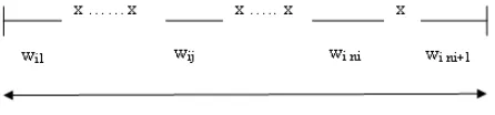
[image:3.612.75.298.235.287.2]We build a single model for a particular term in a given corpus. Let us suppose the term under consid-eration isx as shown in Figure 1. We describe the notation for a particular document,iin the corpus.
Figure 1: The document structure and the gaps be-tween terms
• di denotes the number of words in document i
(i.e. the document length).
• ni denotes the number of occurrences of term
xin documenti.
• wi1denotes the position of the first occurrence of termxin documenti.
• wi2, . . . , wini denotes the successive gaps
be-tween occurrences of termxin documenti.
• wini+1denotes the gap for the next occurrence
ofx, somewhere after the document ends.
• ceni is the value at which observation wini+1
is censored, as explained in section 3.2.2.
3.2 The Model
We suppose we are looking through a document, noting when the term of interest occurs. Our model assumes that the term occurs at some low underly-ing base rate1/λ1 but, after the term has occurred, then the probability of it occurring soon afterwards is increased to some higher rate1/λ2. Specifically, the rate of re-occurrence is modeled by a mixture of two exponential distributions. Each of the exponen-tial components is described as follows:
• The exponential component with larger mean (average),1/λ1, determines the rate with which the particular term will occur if it has not oc-curred before or it has not ococ-curred recently.
• The second component with smaller mean (average), 1/λ2, determines the rate of re-occurrence in a document or text chunk given that it has already occurred recently. This com-ponent captures the bursty nature of the term in the text (or document) i.e. the within-document
burstiness.
The mixture model is described as follows:
φ(wij) = pλ1e−λ1wij+ (1−p)λ2e−λ2wij
forj ∈ {2, . . . , ni}. pand(1−p)denote respec-tively, the probabilities of membership for the first and the second exponential distribution.
There are a few boundary conditions that the model is expected to handle. We take each of these cases and discuss them briefly:
3.2.1 First occurrence
The model treats the first occurrence of a term dif-ferently from the other gaps. The second exponen-tial component measuring burstiness does not fea-ture in it. Hence the distribution is:
φ1(wi1) = λ1e−λ1wi1
3.2.2 Censoring
Here we discuss the modeling of two cases that require special attention, corresponding to gaps that have a minimum length but whose actual length is unknown. These cases are:
• The last occurrence of a term in a document.
• The term does not occur in a document at all.
In our case, we assume the particular term would eventually occur, but the document has ended before it occurs so we do not observe it. In our notation we observe the termnitimes, so the(ni+ 1)thtime the term occurs is after the end of the document. Hence the distribution ofwini+1is censored at lengthceni.
If ceni is small, so that the nthi occurrence of the term is near the end of the document, then it is not surprising thatwini+1is censored. In contrast ifceni
is large, so the nthi occurrence is far from the end of the document, then either it is surprising that the term did not re-occur, or it suggests the term is rare. The information about the model parameters that is given by the censored occurrence is,
P r(wini+1 > ceni) = ∞
ceni
φ(x)dx
=pe−λ1ceni+ (1−p)e−λ2ceni; where,
ceni = di− ni
j=1
wij
Also when a particular term does not occur in a document, our model assumes that the term would eventually occur had the document continued indef-initely. In this case the first occurrence is censored and censoring takes place at the document length. If a term does not occur in a long document, it suggests the term is rare.
3.3 Bayesian formulation
Our modeling is based on a Bayesian approach (Gel-man et al., 1995). The Bayesian approach differs from the traditional frequentist approach. In the fre-quentist approach it is assumed that the parameters of a distribution are constant and the data varies. In the Bayesian approach one can assign distrib-utions to the parameters in a model. We choose non-informative priors, as is common practice in Bayesian applications. So we put,
p∼U nif orm(0,1), and
λ1∼U nif orm(0,1)
To tell the model thatλ2 is the larger of the twoλs, we putλ2=λ1+γ, whereγ >0, and
γ ∼U nif orm(0,1)
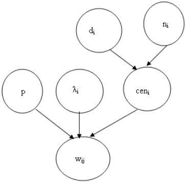
[image:4.612.335.517.56.237.2]Also ceni depends on the document length di and the number of occurrences of the term in that doc-ument, ni. Fitting mixture techniques is tricky and
Figure 2: Bayesian dependencies between the para-meters
requires special methods. We use data augmenta-tion to make it feasible to fit the model using Gibbs Sampling (section 4.2). For details about this, see Robert (1996) who describes in detail the fitting of mixture models in MCMC methods (section 4.2).
4 Parameter Estimation
4.1 Bayesian Estimation
In the Bayesian approach of parameter estimation, the parameters are uncertain, and it is assumed that they follow some distribution. In our case the para-meters and the data are defined as:
Θ ={p, λ1, λ2}denote the parameters of the model.
W ={wi1, . . . , wini, wini+1}denotes the data.
Hence based on this we may define the following:
• f(Θ) is the prior distribution ofΘ as assigned in section 3.3. It summarizes everything we know aboutΘ apart from the dataW .
• f(W |Θ) is the likelihood function. It is our model for the dataW conditional on the para-metersΘ. (As well as the observed data, the likelihood also conveys the information given by the censored values)
Deriving the density function for a parameter setΘ after observing dataW , can be achieved by using
Bayes Theorem as:
f(Θ|W ) = f(W |Θ) f(Θ)
f(W ) (1)
wheref(W )is simply a normalizing constant, inde-pendent ofΘ. It can be computed in terms of the likelihood and prior as:
f(W ) =
f(W |Θ) f(Θ) dΘ
Hence equation 1 is reduced to:
f(Θ|W )∝f(W |Θ) f(Θ)
So, once we have specified the posterior density functionf(Θ|W ), we can obtain the estimates of the parametersΘ by simply averaging the values gener-ated byf(Θ|W ).
4.2 Gibbs Sampling
The density function of Θi, f(Θi|W ) can be ob-tained by integrating f(Θ|W ) over the remaining parameters ofΘ. But in many cases, as in ours, it is impossible to find a closed form solution off(Θi).
In such cases we may use a simulation process based on random numbers, Markov Chain Monte
Carlo (MCMC) (Gilks et al., 1996). By generating
a large sample of observations from the joint distri-bution f(Θ, W), the integrals of the complex dis-tributions can be approximated from the generated data. The values are generated based on the Markov chain assumption, which states that the next gener-ated value only depends on the present value and does not depend on the values previous to it. Based on mild regularity conditions, the chain will gradu-ally forget its initial starting point and will eventu-ally converge to a unique stationary distribution.
Gibbs Sampling (Gilks et al., 1996) is a popular
method used for MCMC analysis. It provides an ele-gant way for sampling from the joint distributions of multiple variables: sample repeatedly from the dis-tributions of one-dimensional conditionals given the current observations. Initial random values are as-signed to each of the parameters. And then these val-ues are updated iteratively based on the joint distri-bution, until the values settle down and converge to
a stationary distribution. The values generated from the start to the point where the chain settles down are discarded and are called the burn-in values. The pa-rameter estimates are based on the values generated thereafter.
5 Results
Parameter estimation was carried out using Gibb’s Sampling on the WinBUGS software (Spiegelhalter et al., 2003). Values from the first 1000 iteration were discarded as burn-in. It had been observed that in most cases the chain reached the stationary distri-bution well within1000iterations. A further5000 it-erations were run to obtain the parameter estimates.
5.1 Interpretation of Parameters
The parameters of the model can be interpreted in the following manner:
• λ1 = 1/λ1 is the mean of an exponential dis-tribution with parameterλ1. λ1 measures the rate at which this term is expected in a running text corpus. λ1 determines the rarity of a term in a corpus, as it is the average gap at which the term occurs if it has not occurred recently. Thus, a large value ofλ1 tells us that the term is very rare in the corpus and vice-versa.
• Similarly, λ2 measures the within-document
burstiness, i.e. the rate of occurrence of a term
given that it has occurred recently. It measures the term re-occurrence rate in a burst within a document. Small values ofλ2 indicate the bursty nature of the term.
• pand1−pdenote, respectively, the probabil-ities of the term occurring with rateλ1 andλ2 in the entire corpus.
Table 1 presents some heuristics for drawing in-ference based on the values of the parameter esti-mates.
5.2 Data
We choose for evaluation, terms from the
Associ-ated Press (AP) newswire articles, as this is a
λ1small λ
1large
λ2small frequently occur-ring and common function word
topical content word occurring in bursts
λ2large comparatively
frequent but well-spaced function word
[image:6.612.316.538.54.287.2]infrequent and scat-tered function word
Table 1: Heuristics for inference, based on the para-meter estimates.
and Sch¨utze, 1999; Umemura and Church, 2000) with respect to modeling different distribution, so as to present a comparative picture. For building the model we randomly selected 1%of the documents from the corpus, as the software (Spiegelhalter et al., 2003) we used is Windows PC based and could not handle enormous volume of data with our available hardware resources. As stated earlier, our model can handle both frequent function terms and rare content terms. We chose terms suitable for demonstrating this. We also used some medium frequency terms to demonstrate their characteristics.
5.3 Parameter estimates
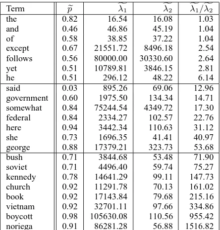
Table 2 shows the parameter estimates for the cho-sen terms. The table does not show the values of
1−pas they can be obtained from the value ofp. It has been observed that the valueλ1/λ2is a good in-dicator of the nature of terms, hence the rows in the table containing terms are sorted on the basis of that value. The table is divided into three parts. The top part contains very frequent (function) words. The second part contains terms in the medium frequency range. And the bottom part contains rarely occurring and content terms.
5.4 Discussion
The top part of the table consists of the very quently occurring function words occurring fre-quently throughout the corpus. These statements are supported by the low values ofλ1 andλ2. These values are quite close, indicating that the occurrence of these terms shows low burstiness in a running text chunk. This supports our heuristics about the value of λ1/λ2, which is small for such terms. Moder-ate, not very high values ofpalso support this state-ment, as the term is then quite likely to be
gener-Term p
λ1 λ
2 λ
1/λ
2
the 0.82 16.54 16.08 1.03
and 0.46 46.86 45.19 1.04
of 0.58 38.85 37.22 1.04
except 0.67 21551.72 8496.18 2.54 follows 0.56 80000.00 30330.60 2.64
yet 0.51 10789.81 3846.15 2.81
he 0.51 296.12 48.22 6.14
said 0.03 895.26 69.06 12.96
government 0.60 1975.50 134.34 14.71 somewhat 0.84 75244.54 4349.72 17.30 federal 0.84 2334.27 102.57 22.76
here 0.94 3442.34 110.63 31.12
she 0.73 1696.35 41.41 40.97
george 0.88 17379.21 323.73 53.68
bush 0.71 3844.68 53.48 71.90
soviet 0.71 4496.40 59.74 75.27
kennedy 0.78 14641.29 99.11 147.73 church 0.92 11291.78 70.13 161.02
book 0.92 17143.84 79.68 215.16
vietnam 0.92 32701.11 97.66 334.86 boycott 0.98 105630.08 110.56 955.42 noriega 0.91 86281.28 56.88 1516.82
Table 2: Parameter estimates of the model for some selected terms, sorted by theλ1/λ2value
ated from either of the exponential distributions (the has high value of p, but since the values of λ are so close, it doesn’t really matter which distribution generated the observation). We observe compara-tively larger values ofλ1 for terms like yet, follows and except since they have some dependence on the document topic. One may claim that these are some outliers having large values of bothλ1 andλ2. The large value ofλ1can be explained, as these terms are rarely occurring function words in the corpus. They do not occur in bursts and their occurrences are scat-tered, so values ofλ2are also large (Table 1). Inter-estingly, based on our heuristics these large values nullify each other to obtain a small value ofλ1/λ2. But since these cases are exceptional, they find their place on the boundary region of the division.
The second part of the table contains mostly
non-topical content terms as defined in the literature
(Katz, 1996). They do not describe the main topic of the document, but some useful aspects of the doc-ument or a nearby topical term. Special attention may be given to the term george, which describes the topical term bush. In a document about George
Bush, the complete name is mentioned possibly only
[image:6.612.79.292.56.146.2]as-signed as a topical term, but not george. The term
government in the group refers to some newswire
article about some government in any state or any country, future references to which are made us-ing this term. Similarly the term federal is used to make future references to the US Government. As the words federal and government are used fre-quently for referencing, they exhibit comparatively small values ofλ2. We were surprised by the occur-rence of terms like said, here and she in the second group, as they are commonly considered as func-tion words. Closer examinafunc-tion revealed the details.
Said has some dependence on the document genre,
with respect to the content and reporting style. The data were based on newswire articles about impor-tant people and events. It is true, though unfor-tunate, that the majority of such people are male, hence there are more articles about men than women (he occurs757,301times in163,884documents as the13th most frequent term in the corpus, whereas
she occurs 164,030 times in48,794 documents as the 70th frequent term). This explains why he has a smaller value ofλ1 than she. But theλ2 values for both of them are quite close, showing that they have similar usage pattern. Again, newswire articles are mostly about people and events, and rarely about some location, referenced by the term here. This ex-plains the large value ofλ1for here. Again, because of its usage for referencing, it re-occurs frequently while describing a particular location, leading to a small value ofλ2. Possibly, in a collection of “travel documents”, here will have a smaller value ofλ1and thus occur higher up in the list, which would allow the model to be used for characterizing genre.
Terms in the third part, as expected, are topical
content terms. An occurrence of such a term
de-fines the topic or the main content word of the doc-ument or the text chunk under consideration. These terms are rare in the entire corpus, and only appear in documents that are about this term, resulting in very high values ofλ1. Also low values of λ2 for these terms mean that repeat occurrences within the same document are quite frequent; the characteris-tic expected from a topical content term. Because of these characteristics, based on our heuristics these terms have very high values ofλ1/λ2, and hence are considered the most informative terms in the corpus.
5.5 Case Studies
Here we study selected terms based on our model. These terms have been studied before by other re-searchers. We study these terms to compare our findings with previous work and also demonstrate the range of inferences that may be derived from our model.
5.5.1 somewhat vrs boycott
These terms occur an approximately equal num-ber of times in the AP corpus, and inverse
doc-ument frequency was used to distinguish between
them (Church and Gale, 1995a). Our model also gives approximately similar rates of occurrence (λ1) for these two terms as shown in Table 2. But the re-occurrence rate,λ2, is110.56 for boycott, which is very small in comparison with the value of4349.72
for somewhat. Hence based on this, our model as-signs somewhat as a rare function word occurring in a scattered manner over the entire corpus. Whereas
boycott is assigned as a topical content word, as it
should be.
5.5.2 follows vrs soviet
These terms were studied in connection with fit-ting Poisson distributions to their term distribution (Manning and Sch¨utze, 1999), and hence determin-ing their characteristics1. In our model, follows has large values of bothλ1 andλ2 (Table 2), so that it has the characteristics of a rare function word. But
soviet has a largeλ1value and a very smallλ2value, so that it has the characteristics of a topical content word. So the findings from our model agree with the original work.
5.5.3 kennedy vrs except
Both these terms have nearly equal inverse
doc-ument frequency for the AP corpus (Church, 2000;
Umemura and Church, 2000) and will be assigned equal weight. They used a method (Kwok, 1996) based on average-term frequency to determine the nature of the term. According to our model, theλ2 value of kennedy is very small as compared to that for except. Hence using theλ1/λ2 measure, we can correctly identify kennedy as a topical content term
1
and except as an infrequent function word. This is in agreement with the findings of the original analysis.
5.5.4 noriega and said
These terms were studied in the context of an adaptive language model to demonstrate the fact that the probability of a repeat occurrence of a term in a document defies the “bag of words” independence assumption (Church, 2000). The deviation from in-dependence is greater for content terms like noriega as compared to general terms like said. This can be explained in the context of our model as said has small values ofλ1andλ2, and their values are quite close to each other (as compared to other terms, see Table 2). Hence said is distributed more evenly in the corpus than noriega. Therefore, noriega defies the independence assumption to a much greater ex-tent than said. Hence their findings (Church, 2000) are well explained by our model.
6 Conclusion
In this paper we present a model for term re-occurrence in text based on gaps between succes-sive occurrences of a term in a document. Parameter estimates based on this model reveal various charac-teristics of term use in a collection. The model can differentiate a term’s dependence on genre and col-lection and we intend to investigate use of the model for purposes like genre detection, corpus profiling, authorship attribution, text classification, etc. The proposed measure of λ1/λ2 can be appropriately adopted as a means of feature selection that takes into account the term’s occurrence pattern in a cor-pus. We can capture both within-document bursti-ness and rate of occurrence of a term in a single model.
References
A. Bookstein and D.R Swanson. 1974. Probabilistic models for automatic indexing. Journal of the
Ameri-can Society for Information Science, 25:312–318.
K. Church and W. Gale. 1995a. Inverse document fre-quency (idf): A measure of deviation from poisson. In Proceedings of the Third Workshop on Very Large
Corpora, pages 121–130.
K. Church and W. Gale. 1995b. Poisson mixtures.
Nat-ural Language Engineering, 1(2):163–190.
K. Church. 2000. Empirical estimates of adaptation: The chance of two noriega’s is closer to p/2 thanp2. In
COLING, pages 173–179.
Anne De Roeck, Avik Sarkar, and Paul H Garthwaite. 2004a. Defeating the homogeneity assumption. In
Proceedings of 7th International Conference on the Statistical Analysis of Textual Data (JADT), pages
282–294.
Anne De Roeck, Avik Sarkar, and Paul H Garthwaite. 2004b. Frequent term distribution measures for dataset profiling. In Proceedings of the 4th
Interna-tional conference of Language Resources and Evalua-tion (LREC), pages 1647–1650.
Alexander Franz. 1997. Independence assumptions con-sidered harmful. In Proceedings of the eighth
confer-ence on European chapter of the Association for Com-putational Linguistics, pages 182–189.
A. Gelman, J. Carlin, H.S. Stern, and D.B. Rubin. 1995.
Bayesian Data Analysis. Chapman and Hall, London,
UK.
W.R. Gilks, S. Richardson, and D.J. Spiegelhalter. 1996.
Markov Chain Monte Carlo in Practice.
Interdisci-plinary Statistics Series. Chapman and Hall, London, UK.
Slava M. Katz. 1996. Distribution of content words and phrases in text and language modelling. Natural
Lan-guage Engineering, 2(1):15–60.
A Kilgarriff. 1997. Using word frequency lists to mea-sure corpus homogeneity and similarity between cor-pora. In Proceedings of ACL-SIGDAT Workshop on
very large corpora, Hong Kong.
K. L. Kwok. 1996. A new method of weighting query terms for ad-hoc retrieval. In SIGIR, pages 187–195.
Christopher D. Manning and Hinrich Sch¨utze. 1999.
Foundations of Statistical Natural Language Process-ing. The MIT Press, Cambridge, Massachusetts.
Christian. P. Robert. 1996. Mixtures of distributions: in-ference and estimation. In W.R. Gilks, S. Richardson, and D.J. Spiegelhalter, editors, Markov Chain Monte
Carlo in Practice, pages 441–464.
D.J. Spiegelhalter, A. Thomas, N. G. Best, and D. Lunn. 2003. Winbugs: Windows version of bayesian infer-ence using gibbs sampling, version 1.4.
K. Umemura and K. Church. 2000. Empirical term weighting and expansion frequency. In Empirical