4890
Conditional Word Embedding and Hypothesis Testing via
Bayes-by-Backprop
Rujun Han
Information Sciences Institute University of Southern California
Arthur Spirling Center for Data Science
New York University [email protected]
Michael Gill Center for Data Science
New York University [email protected]
Kyunghyun Cho Center for Data Science
New York University CIFAR Global Scholar [email protected]
Abstract
Conventional word embedding models do not leverage information from document meta-data, and they do not model uncertainty. We address these concerns with a model that incorporates document covariates to es-timate conditional word embedding distribu-tions. Our model allows for (a) hypothesis tests about the meanings of terms, (b) assess-ments as to whether a word is near or far from another conditioned on different covariate val-ues, and (c) assessments as to whether esti-mated differences are statistically significant.
1 Introduction
Whether a word’s meaning varies across contexts has become a major focus of NLP, linguistics, and social science research in recent years. For exam-ple, since the early 20th century, the word “gay” has evolved from describing an emotion to be-ing more aligned with sexual orientation ( Hamil-ton et al.,2016b). Popular word embedding tech-niques (e.g., Mikolov et al., 2013a; Pennington et al.,2014) have proven useful for analyzing lan-guage evolution. But to use these models for such research, scholars often divide a corpus into dis-tinct training sets (e.g., train independent language models on different decades of text) and compare model output across specifications in an ad hoc
way (Garg et al., 2018). Such splitting inhibits many within- and across-word comparisons, since embeddings are only comparable within a given model. Additionally, most methods ignore the
variance of words, mechanically treating words equally regardless of the volatility, or uncertainty, in their meanings. If one inspects semantics with only point estimates of embeddings, it is hard to tell whether embeddings represent meaningful traits or are simply noise in the data.
We address these concerns in three ways. First, we estimate a vector for each distinct value of the
document covariates, using a multilayer percep-tron (MLP) with a non-linear activation function. Second, we parametrize the covariance matrix of each embedding vector explicitly in the model, adopting the Bayes-by-Backprop algorithm ( Blun-dell et al., 2015). Third, we utilize HotellingT2
statistics (Hotelling,1931) to assess whether esti-mated differences in word vectors are statistically differentiable under a null χ2 distribution (Ito,
1956). To our knowledge, no prior work evaluates word embeddings with this statistical framework.
2 Related Work
Drift Analysis using Word Embeddings There are several ways to measure drifts in word mean-ings. Hamilton et al.(2016c) propose the use of cosine similarities of words in different contexts to detect changes. Hamilton et al. (2016b) pro-vide an alternative measure based on the distance of words from their nearest neighbors. Rudolph and Blei (2018) analyze absolute drift of words using Euclidean distance in (two discrete) slices of data. All of these methods compute the word distance based only on the point (i.e., mean) esti-mates of the word embeddings.
Conditional Word Embedding Rudolph and Blei (2018) estimate dynamic Bernoulli embed-dings (DBE), extending the exponential family embedding (Rudolph et al., 2016) generalization of Mikolov et al. (2013a), to learn conditional word embeddings over time. Their amortized approach builds a separate neural network that transforms a global word vector into a covariate-specific vector, and is closely related to our ap-proach in this paper. However, a noticeable omis-sion in their model is that they do not explicitly model parameter covariance or uncertainty.
energy-based learning framework in which each word is represented as a multivariate Gaussian distribu-tion with a diagonal covariance. The energy func-tion is defined by the divergence (e.g., KL) be-tween two Gaussian embeddings, and the mar-gin ranking loss (Weston et al., 2011) is mini-mized. A related model is the Bayesian skip-gram inBrazinskas et al.(2017), which posits a genera-tive model where words are associated with multi-variate Gaussian latent variables that generate con-text words. The parameters of those prior distri-butions over the multivariate Gaussian latent vari-ables are estimated by maximizing the variational lowerbound, and act as word embeddings.
These works replace mean estimates of embed-dings with Gaussian distributions, similar to our proposal here. However, they arrive at this dif-ferently; Vilnis and McCallum (2017) from the energy-based learning (LeCun et al., 2006), and
Brazinskas et al.(2017) from generative modeling. We provide yet another angle: via (approximate) Bayesian neural networks.
3 Conditional Word Embedding
Adopting Bayes-by-Backprop for Estimation
Given a tuple of a word v, a covariate x and a context word vc, we define the conditional log-probability as
logp(vc|v, x) =θv>|xθ c vc−log
X
v0
c∈V
expθ>v|xθcv0
c
,
where θv|x andθcvc are the conditional word
em-bedding ofvgivenxand the context embedding of
vc, respectively. V is the vocabulary of all unique words. To avoid the expensive computation of the partition function, we use negative sampling (Mikolov et al., 2013b), which stochastically ap-proximates the log-probability above by:
logp(vc|v, x)≈logσ(θ>v|xθcvc) (1)
+ 1
M
M X
m=1
log(1−σ(θv>|xθcvm c )),
wherevcm∈V is them-th negative sample drawn from a unigram distribution estimated fromD.
We define a prior distribution over each param-eterθto be a scaled mixture of two Gaussians, as suggested byBlundell et al.(2015):
logp(θi) = log uN(θi|0, σ21) (2)
+(1−u)N(θi|0, σ22)
,
whereσ1,σ2anduare the hyperparameters. As exactly marginalizing out the parametersθ·
and θ·c is not scalable, we maximize the
vari-ational lowerbound of the marginal probability. To do so, we introduce a variational posterior
q(θ|φ) parametrized by its own parameter setφ. Then, the variational lowerbound is defined as
−F(θ, D) = Eq[logp(D|θ)]−KL(q(θ)kp(θ)), wherelogp(D|θ) = P
(v,x,vc)∈Dlogp(vc|v, x)in
our case. This is stochastically approximated by
−F(θ, D)≈ 1
M
M X
m=1
logp(D|θ(m)) (3)
−logq(θ(m)|φ) + logp(θ(m)),
whereθ(m)is them-th sample from the variational posteriorq(Blundell et al.,2015) via the Gaussian reparametrization inKingma and Welling(2013). We formulate the variational posterior as a multi-variate Gaussian with diagonal covariance.
We use stochastic gradient descent (SGD) to minimizeFwith respect to the variational param-etersφ. At each SGD step, we compute the gra-dient of the following per-example cost given an example(v, vc, x)∈D:
f(θ,(v,vc, x))≈ −logp(vc|v, x) + logq(˜θv|x|φ)
+ logq(˜θcvc) + logq(˜θcv0
c)−logp(˜θ),
whereθ˜is a single sample from the approximate posterior, andlogp(vc|v, x)andlogp(˜θ)are from Eqs. (1)–(2). We then estimate the (approximate) posterior distribution of each conditional word embeddingθv|x rather than its point estimate, by minimizing F. See Sec. A of the supplementary material for the detailed steps for computing the per-example cost.
Parametrized Conditional Word Embedding
An issue with the approach described so far is the number of parameters grows linearly in the size of the vocabulary and in the number of covariate par-titions, i.e.,O(|V| × |C|), whereCis the set of all partitions. This effectively excludes any potential sharing of structures underlying words across dif-ferent covariate values and decreases the number of examples per parameter. To avoid this issue, we use a single parametrized function to compute the variational parametersφof each conditional word embeddingθv|x.
without any hidden layer and tanhoutput layer, i.e., the affine transformation followed by point-wisetanh, that takes as input both a global word vectorµ(vv)and a covariate vectorµ(xx)and outputs
µv|x, i.e.,µv|x =fψ( h
µ(vv);µ(xx) i
),whereψis the parameters of this mean-transformation network. The diagonal covariance σv|x is parametrized as
σv|x = log(1 + exp(ρv)), where ρv is a pa-rameter shared across all covariate configurations. We then minimize F w.r.t. these parameters ψ, n
µ(vv), ρv o
v∈V and n
µ(xx) o
x∈C.
This approach of parametrized conditional word embeddings significantly reduces the number of parameters from O(|V| × |C|) toO(|V|+|C|), while maintaining posterior uncertainty of the es-timated conditional word embeddingθv|x.
4 Divergences for Word Embeddings
As we estimate the approximate posterior uncer-tainty of conditional word vectors, we can estimate richer relations between vectors (e.g., KL) in addi-tion to more common comparisons (e.g., cosine or Euclidean distance). Moreover, we can explicitly test for whether two vectors are (un)likely to have the same mean in the population. Below, we intro-duce how Hotelling’sT2 may be used for word-drift or across-word hypothesis testing.
Hotelling’s T2 Statistic We use the estimated posterior mean vector µv|x and the diagonal co-variance vector σv|x of two word-covariate pairs
v|xi and v|xj to compute the T2 statistic, as if they were estimates from two sets of samples:
T2= (µi−µj)>diag(s)−1(µi−µj). The pooled (diagonal) covariancesof word pairs is computed
by s = (ni−1)·σ
2
i+(nj−1)·σ
2
j
ni+nj−2 , whereni andnj are
the numbers of occurrences ofv|xiandv|xj inD, respectively.1 Unlike other divergence measures, this T2 statistic explicitly takes into account the frequencies of the word-covariate pairs.
Under general conditions, e.g., Dis large, the sampling distribution ofT2converges to aχ2d dis-tribution (Ito,1956) withdequal to the embedding dimensionality. This allows us to statistically test such a null hypothesis as Diff(vi|x, vj|x) = 0and Diff(v|xi, v|xj) = 0.
5 Application: Political Speech in UK
Data We use U.K. Parliament speech records from 1935-2012 as our training data (Rheault
[image:3.595.322.510.65.186.2]1T2is valid only whenni>1andnj>1.
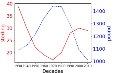
Figure 1: The ranks of “sterling” (solid line) and “pound” (dotted line) w.r.t. “currency” across the decades according to KL divergence.
et al.,2016). Our conditioning variable of interest is the decade in which a speech occurred. More details are in Sec. B of the supplementary file.
Model and Learning For each word in the cor-pus, we consider six surrounding words as its con-text. The size of embedding is set to 100. We use six negative samples to compute Eq. (1). We use Adagrad (Duchi et al., 2011) with the initial learning rate0.05for learning.2 For other hyper-parameters, see the supplementary material. We refer to our approach by BBP. For comparison, we also train analogous DBE embeddings using code from the authors.
6 Result and Analysis
Impact of Covariates To demonstrate how doc-ument covariates influence conditional word em-beddings, we compare the vector for “currency” against “sterling” and “pound” according to the KL divergence in each decade, which is shown in Fig.1. In each time period we report the ranking of each w.r.t “currency”. Here, we observe that piv-otal points for both “sterling” and “pound” occur in the 1970s, which coincides with the moment the UK began to abandon the ‘sterling area’ (Part III in Schenk,2010). As such, this financial policy appears to have encouraged semantic drift of the word “pound” towards “currency”. See Sec. D in the supplementary material for more details.
We also show a few more examples in Figure 2 and Figure 3 from the Dictionary Induction section below.
Dictionary Induction As a quantitative com-parison between the proposed approach and the DBE, we take a dictionary of (British) political terms byLaver and Garry(2000) and look at the
Figure 2: The ranks between “market” and “money” across the decades according to KL di-vergence.
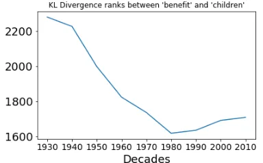
Figure 3: The ranks between “benefit” and “chil-dren” across the decades according to KL diver-gence.
average pair-wise, directional rank in each cate-gory (“pro-state”, “con-state” and “neutral-state”). We only consider the 2,000 most frequent words in the vocabulary and embeddings with the covari-ate (decade) set to 2000s. We observed that the proposed model using KL divergence has signif-icantly smaller average pair-wise ranks in “pro-state” (4052 vs. 5047) and “con-“pro-state” (2578 vs. 3758) while performs slightly worse than DBE in “neutral-state” category (5414 vs. 5031) suggest-ing that the proposal approach can cluster words from similar semantic group into closer neighbors than DBE.
Furthermore, we pick 5 most frequent words from “pro-state” and “con-state” and show their average pair-wise rankings and percentile in Table 1. Out of 25K words, our proposed model is able to rank most chosen words within top 10% per-centile.
Statistical Word Drift Analysis Our BBP ap-proach permits meaningful downstream hypothe-sis tests of word drift, i.e, Diff(v|xi, v|xj) = 0, and across-word similarity, i.e., Diff(vi, vj) = 0. Among the 2,000 most frequent words in our
sam-Pro-state Con-state
Words Ranks Pctl Words Ranks Pctl benefit 1437 5.7 market 1783 7.1 children 2432 9.8 money 1623 6.5
education 716 2.9 own 2852 11.4
[image:4.595.310.523.194.267.2]health 996 4.0 private 1670 6.7 transport 4247 17.0 value 1693 6.8
Table 1: Average pair-wise rankings of most fre-quent words in “pro-state” and “con-state” from a British political dictionary.
DBE No Covariance Covariance
Words Ranks L2 cosine KL T2
uk 1 1.60 0.81 61.4 99.7
eu 2 1.58 0.84 44.6 89.2
war 6 1.52 0.85 48.4 96.8
council 8 1.66 0.84 71.0 142.0∗∗ labour 15 1.63 0.82 62.4 124.8∗
Table 2: Top word drifts selected based on DBE model and estimated by BBP. * and ** indicate p-value≤0.05and0.01, respectively.
ple, we perform hypothesis tests of word drifts, comparing vectors from the 1940s against those from the 2000s. We compare results from BBP against the top-100 estimated drifts via DBE. We first observe that most of the top-ranked words by L2 distance in the DBE model are not statistically significant. With the p-value threshold ofα= 0.1, only eleven words were deemed to have had sig-nificant drift, including “council”, “labour”, “eu-ropean” and “defence”. Sec. E of the supplement includes entire lists of this drift analysis.
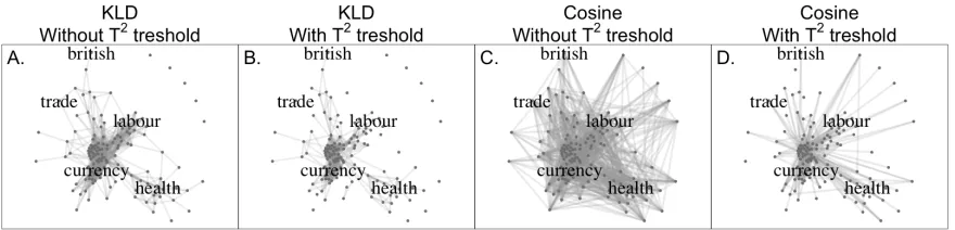
[image:4.595.84.276.246.365.2]Figure 4: Semantic Graphs with KLD vs. Cosine Similarity
Cosine Similarity vs. KL Divergence In con-trast to cosine distance, our proposed method al-lows computation of the KLD between two vec-tors that takes into account their covariance. Fig-ure 2 presents semantic graphs estimated in the spirit ofHamilton et al.(2016a). The set of words is given by the union set of the 10 nearest neigh-bors, measured by cosine similarity and KLD, for the five seed words: “currency”, “british”, “health”, “trade” and “labour”. This results in 130 unique words including the seed words and we compute their pair-wise KLD matrix, WKL and pairwise cosine similarity matrix, Wcos. We convert WKL to a symmetric matrix as WKL0 =
(WKL+WKLT )/2. BothWKL andWcoshave di-mensions of130×130.
Edge weights in Figures 2.A and 2.B are computed by taking a sigmoid transfor-mation of normalized entries in WKL0 , i.e.,
σ(normalize(w0KL
i,j)). Edge weights in 2.C and
2.D are computed by arccos(wcosi,j), following
Hamilton et al. (2016a). Edges with weights below 90th percentiles are dropped for visual clarity. Note that with the same number of edges being eliminated, the KLD charts appear more clustered around seed words, implying that incorporating covariance matrix creates useful segregation of words within local contexts; graphs constructed via cosine similarity seem to disperse edge weights in a more diffuse manner.
T2-based Significance In the context of uncertainty-aware word embeddings, we can use theT2 statistic to filter out additional words from a nearest neighbor set. For instance, in Figure 2.B and 2.D, we drop edges for word pairs that fall below the 90th percentile of computed T2 statistics. Filtering with Hotelling T2 results in more sparse semantic graphs.
7 Conclusion
We proposed an uncertainty-aware conditional word embedding model that combines two ideas; (1) variational Bayesian learning for estimating parameter uncertainty, and (2) structured embed-dings conditioned on covariates. This provides a principled direction to investigate hypothesis tests of word vectors in various forms. We evaluated various aspects of the proposed approach on U.K. Parliament speech records from 1935-2012. We believe the proposed approach will serve as a more rigorous tool in social science and other domains.
8 Acknowledgments
KC thanks the support by eBay, TenCent, NVIDIA and CIFAR. RH thanks the support by MINDS re-search group at Information Sciences Institute of University of California.
References
Charles Blundell, Julien Cornebise, Koray Kavukcuoglu, and Daan Wierstra. 2015. Weight uncertainty in neural networks.arXiv, 1505.05424.
Arthur Brazinskas, Serhii Havrylov, and Ivan Titov. 2017. Embedding words as distributions with a bayesian skip-gram model. arXiv, 1711.11027.
John Duchi, Elad Hazan, and Yoram Singer. 2011. Adaptive subgradient methods for online learning and stochastic optimization. Journal of Machine Learning Research, 12(Jul):2121–2159.
Nikhil Garg, Londa Schiebinger, Dan Jurafsky, and James Zou. 2018. Word embeddings quantify 100 years of gender and ethnic stereotypes. Proceed-ings of the National Academy of Sciences (Preprint), pages 1–10.
William L Hamilton, Jure Leskovec, and Dan Jurafsky. 2016b. Cultural shift or linguistic drift? comparing two computational measures of semantic change. In Proceedings of the Conference on Empirical Meth-ods in Natural Language Processing. Conference on Empirical Methods in Natural Language Process-ing, volume 2016, page 2116. NIH Public Access.
William L. Hamilton, Jure Leskovec, and Dan Jurafsky. 2016c. Diachronic word embeddings reveal statisti-cal laws of semantic change. arXiv, 1605.09096v4.
Harold Hotelling. 1931. The generalization of stu-dent’s ratio. The Annals of Mathematical Statistics, 2(3):360–378.
Koichi Ito. 1956. Asymptotic formulae for the distribu-tion of hotelling’s generalizedt20statistic. The An-nals of Mathematical Statistics, 27(4):1091–1105.
Diederik P Kingma and Max Welling. 2013. Auto-encoding variational bayes. arXiv preprint arXiv:1312.6114.
Michael Laver and John Garry. 2000. Estimating pol-icy positions from political texts. American Journal of Political Science, pages 619–634.
Yann LeCun, Sumit Chopra, Raia Hadsell, M Ranzato, and F Huang. 2006. A tutorial on energy-based learning.Predicting structured data.
Tomas Mikolov, Kai Chen, Greg Corrado, and Jef-frey Dean. 2013a. Efficient estimation of word representations in vector space. arXiv preprint arXiv:1301.3781.
Tomas Mikolov, Ilya Sutskever, Kai Chen, Greg Cor-rado, and Jeffrey Dean. 2013b. Distributed repre-sentations of words and phrases and their composi-tionality.arXiv, 1310.4546.
Jeffrey Pennington, Richard Socher, and Christopher Manning. 2014. Glove: Global vectors for word representation. InProceedings of the 2014 confer-ence on empirical methods in natural language pro-cessing (EMNLP), pages 1532–1543.
Ludovic Rheault, Kaspar Beelen, Christopher Cochrane, and Graeme Hirst. 2016. Measuring emotion in parliamentary debates with automated textual analysis. PloS one, 11(12):e0168843.
Maja Rudolph and David Blei. 2018. Dynamic embed-dings for language evolution. InWWW 2018: The 2018 Web Conference, volume April 23–27, 2018, pages 1003–1011.
Maja Rudolph, Francisco Ruiz, Stephan Mandt, and David Blei. 2016. Exponential family embeddings. InAdvances in Neural Information Processing Sys-tems, pages 478–486.
Catherine R Schenk. 2010. The decline of sterling: managing the retreat of an international currency, 1945–1992. Cambridge University Press.
Luke Vilnis and Andrew McCallum. 2017. Word representations via gaussian embedding. arXiv, 1412.6623.