Better Word Representations with Recursive Neural Networks for Morphology

Better Word Representations with Recursive Neural Networks for

Morphology

Minh-Thang Luong Richard Socher Christopher D. Manning Computer Science Department Stanford University, Stanford, CA, 94305

{lmthang, manning_}@stanford.edu richard@socher.org

Abstract

Vector-space word representations have been very successful in recent years at im-proving performance across a variety of NLP tasks. However, common to most existing work, words are regarded as in-dependent entities without any explicit re-lationship among morphologically related words being modeled. As a result, rare and complex words are often poorly estimated, and all unknown words are represented in a rather crude way using only one or a few vectors. This paper addresses this shortcoming by proposing a novel model that is capable of building representations for morphologically complex words from their morphemes. We combine recursive neural networks (RNNs), where each mor-pheme is a basic unit, with neural language models (NLMs) to consider contextual information in learning morphologically-aware word representations. Our learned models outperform existing word repre-sentations by a good margin on word sim-ilarity tasks across many datasets, includ-ing a new dataset we introduce focused on rare words to complement existing ones in an interesting way.

1 Introduction

The use of word representations or word clusters pretrained in an unsupervised fashion from lots of text has become a key “secret sauce” for the suc-cess of many NLP systems in recent years, across tasks including named entity recognition, part-of-speech tagging, parsing, and semantic role label-ing. This is particularly true in deep neural net-work models (Collobert et al., 2011), but it is also true in conventional feature-based models (Koo et al., 2008; Ratinov and Roth, 2009).

Deep learning systems give each word a distributed representation, i.e., a dense low-dimensional real-valued vector or an embedding. The main advantage of having such a distributed representation over word classes is that it can cap-ture various dimensions of both semantic and syn-tactic information in a vector where each dimen-sion corresponds to a latent feature of the word. As a result, a distributed representation is compact, less susceptible to data sparsity, and can implicitly represent an exponential number of word clusters. However, despite the widespread use of word clusters and word embeddings, and despite much work on improving the learning of word repre-sentations, from feed-forward networks (Bengio et al., 2003) to hierarchical models (Morin, 2005; Mnih and Hinton, 2009) and recently recurrent neural networks (Mikolov et al., 2010; Mikolov et al., 2011), these approaches treat each full-form word as an independent entity and fail to cap-ture the explicit relationship among morphologi-cal variants of a word.1 _{The fact that}

morphologi-cally complex words are often rare exacerbates the problem. Though existing clusterings and embed-dings represent well frequent words, such as “dis-tinct”, they often badly model rare ones, such as “distinctiveness”.

In this work, we use recursive neural networks (Socher et al., 2011b), in a novel way to model morphology and its compositionality. Essentially, we treat each morpheme as a basic unit in the RNNs and construct representations for morpho-logically complex words on the fly from their mor-phemes. By training a neural language model (NLM) and integrating RNN structures for com-plex words, we utilize contextual information in

1_{An almost exception is the word clustering of (Clark,} 2003), which does have a model of morphology to encour-age words ending with the same suffix to appear in the same class, but it still does not capture the relationship between a word and its morphologically derived forms.

an interesting way to learn morphemic semantics and their compositional properties. Our model has the capability of building representations for any new unseen word comprised of known mor-phemes, giving the model an infinite (if still in-complete) covered vocabulary.

Our learned representations outperform pub-licly available embeddings by a good margin on word similarity tasks across many datasets, which include our newly released dataset focusing on rare words (see Section 5). The detailed analysis in Section 6 reveals that our models can blend well syntactic information, i.e., the word structure, and the semantics in grouping related words.2

2 Related Work

Neural network techniques have found success in several NLP tasks recently such as sentiment anal-ysis at the sentence (Socher et al., 2011c) and document level (Glorot et al., 2011), language modeling (Mnih and Hinton, 2007; Mikolov and Zweig, 2012), paraphrase detection (Socher et al., 2011a), discriminative parsing (Collobert, 2011), and tasks involving semantic relations and compo-sitional meaning of phrases (Socher et al., 2012).

Common to many of these works is use of a distributed word representation as the basic input unit. These representations usually capture lo-cal cooccurrence statistics but have also been ex-tended to include document-wide context (Huang et al., 2012). Their main advantage is that they can both be learned unsupervisedly as well as be tuned for supervised tasks. In the former training regiment, they are evaluated by how well they can capture human similarity judgments. They have also been shown to perform well as features for supervised tasks, e.g., NER (Turian et al., 2010).

While much work has focused on different ob-jective functions for training single and multi-word vector representations, very little work has been done to tackle sub-word units and how they can be used to compute syntactic-semantic word vectors. Collobert et al. (2011) enhanced word vectors with additional character-level features such as capitalization but still can not recover more detailed semantics for very rare or unseen words, which is the focus of this work.

This is somewhat ironic, since working out

cor-2_{The rare word dataset and trained word vectors can be} found at _{http://nlp.stanford.edu/˜lmthang/} morphoNLM.

rect morphological inflections was a very central problem in early work in the parallel distributed processing paradigm and criticisms of it (Rumel-hart and McClelland, 1986; Plunkett and March-man, 1991), and later work developed more so-phisticated models of morphological structure and meaning (Gasser and Lee, 1990; Gasser, 1994), while not providing a compositional semantics nor working at the scale of what we present.

To the best of our knowledge, the work clos-est to ours in terms of handing unseen words are the factored NLMs (Alexandrescu and Kirchhoff, 2006) and the compositional distributional seman-tic models (DSMs) (Lazaridou et al., 2013). In the former work, each word is viewed as a vec-tor of features such as stems, morphological tags, and cases, in which a single embedding matrix is used to look up all of these features.3 _Though

this is a principled way of handling new words in NLMs, the by-product word representations, i.e. the concatenations of factor vectors, do not en-code in them the compositional information (they are stored in the NN parameters). Our work does not simply concatenate vectors of morphemes, but rather combines them using RNNs, which cap-tures morphological compositionality.

The latter work experimented with different compositional DSMs, originally designed to learn meanings of phrases, to derive representations for complex words, in which the base unit is the mor-pheme similar to ours. However, their models can only combine a stem with an affix and does not support recursive morpheme composition. It is, however, interesting to compare our neural-based representations with their DSM-derived ones and cross test these models on both our rare word similarity dataset and their nearest neighbor one, which we leave as future work.

Mikolov et al. (2013) examined existing word embeddings and showed that these representations already captured meaningful syntactic and seman-tic regularities such as the singular/plural relation thatx_{apple -} x_apples ≈x_{car -} x_{cars. However,} we believe that these nice relationships will not hold for rare and complex words when their vec-tors are poorly estimated as we analyze in Sec-tion 6. Our model, on the other hand, explicitly represents these regularities through morphologi-cal structures of words.

ƵŶWZ ĨŽƌƚƵŶĂƚĞ^dD

ůLJ^h&

ƵŶĨŽƌƚƵŶĂƚĞůLJ^dD

ܹ௠ǡܾ௠

ܹ௠ǡܾ௠

ƵŶĨŽƌƚƵŶĂƚĞ^dD

Figure 1:Morphological Recursive Neural Net-work. A vector representation for the word “un-fortunately” is constructed from morphemic vec-tors: unpre, fortunatestm, lysuf. Dotted nodes are computed on-the-fly and not in the lexicon.

3 Morphological RNNs

Our morphological Recursive Neural Network (morphoRNN) is similar to (Socher et al., 2011b), but operates at the morpheme level instead of at the word level. Specifically, morphemes, the mini-mum meaning-bearing unit in languages, are mod-eled as real-valued vectors of parameters, and are used to build up more complex words. We assume access to a dictionary of morphemic analyses of words, which will be detailed in Section 4.

Following (Collobert and Weston, 2008), dis-tinct morphemes are encoded by column vectors in a morphemic embedding matrixWe ∈Rd×|M|, wheredis the vector dimension and M is an or-dered set of all morphemes in a language.

As illustrated in Figure 1, vectors of morpho-logically complex words are gradually built up from their morphemic representations. At any lo-cal decision (a dotted node), a new parent word vector (p) is constructed by combining a stem

vec-tor (xstem) and an affix vector (xaffix) as follow:

p=f(Wm[xstem;xaffix] +bm) (1)

Here,Wm∈Rd×2dis a matrix of morphemic pa-rameters whilebm ∈Rd×1 is an intercept vector. We denote an element-wise activation function as f, such astanh. This forms the basis of our mor-phoRNN models withθ ={We,Wm,bm}being the parameters to be learned.

3.1 Context-insensitive Morphological RNN

Our first model examines how well morphoRNNs could construct word vectors simply from the mor-phemic representation without referring to any context information. Input to the model is a refer-ence embedding matrix, i.e. word vectors trained by an NLM such as (Collobert and Weston, 2008)

and (Huang et al., 2012). By assuming that these reference vectors are right, the goal of the model is to construct new representations for morpholog-ically complex words from their morphemes that closely match the corresponding reference ones.

Specifically, the structure of the context-insensitive morphoRNN (cimRNN) is the same as the basic morphoRNN. For learning, we first de-fine a cost function s for each word xi as the

squared Euclidean distance between the newly-constructed representation p_c(xi) and its

refer-encevectorp_r(xi):s(xi) =∥pc(xi)−pr(xi)∥22.

The objective function is then simply the sum of all individual costs overNtraining examples, plus a regularization term, which we try to minimize:

J(θ) =

N

∑

i=1

s(xi) +

λ

2∥θ∥ 2

2 (2)

3.2 Context-sensitive Morphological RNN

The cimRNN model, though simple, is interesting to attest if morphemic semantics could be learned solely from an embedding. However, it is lim-ited in several aspects. Firstly, the model has no chance of improving representations for rare words which might have been poorly estimated. For example, “distinctness” and “unconcerned” are very rare, occurring only 141 and 340 times in Wikipedia documents, even though their corre-sponding stems “distinct” and “concern” are very frequent (35323 and 26080 respectively). Trying to construct exactly those poorly-estimated word vectors might result in a bad model with parame-ters being pushed in wrong directions.

ƵŶĨŽƌƚƵŶĂƚĞůLJ ƚŚĞ ďĂŶŬ ǁĂƐ ĐůŽƐĞĚ ܹǡܾ

ƵŶ ĨŽƌƚƵŶĂƚĞ

ƵŶĨŽƌƚƵŶĂƚĞ ůLJ ĐůŽƐĞ Ě

ܹ௠ǡܾ௠

ܹ௠ǡܾ௠ ܹ௠ǡܾ௠

ݒ

;ďͿ

;ĂͿ

Figure 2:Context-sensitive morphological RNN

has two layers: (a) themorphologicalRNN, which constructs representations for words from their morphemes and (b) the word-based neural lan-guage which optimizes scores for relevant ngrams.

Structure-wise, we stack the NLM on top of our morphoRNN as illustrated in Figure 2. Complex words like “unfortunately” and “closed” are con-structed from their morphemic vectors, unpre + fortunatestm +lysufandclosestm+ dsuf, whereas simple words4_{, i.e. stems, and affixes could be}

looked up from the morphemic embedding ma-trixWeas in standard NLMs. Once vectors of all complex words have been built, the NLM assigns a score for each ngram ni consisting of words

x1, . . . , xnas follows:

s(ni) =υ⊤f(W[x1;. . .;xn] +b)

Here, xj is the vector representing the wordxj.

We follow (Huang et al., 2012) to use a sim-ple feed-forward network with oneh-dimensional hidden layer. W _∈ Rh×nd_{, b ∈ R}h×1_{, and} υ ∈ Rh×1 _{are parameters of the NLM, and f is}

an element-wise activation function as in Eq. (1). We adopt a ranking-type cost in defining our ob-jective function to minimize as below:

J(θ) =

N

∑

i=1

max{0,1−s(ni) +s(ni)} (3)

Here,N is the number of all available ngrams in the training corpus, whereas ni is a “corrupted”

ngram created fromni by replacing its last word

with a random word similar in spirit to (Smith and Eisner, 2005). Our model parameters are

θ=_{We,Wm,bm,W,b,υ}.

Such a ranking criterion influences the model to assign higher scores to valid ngrams than to

4_{“fortunate”, “the”, “bank”, “was”, and “close”.}

invalid ones and has been demonstrated in (Col-lobert et al., 2011) to be both efficient and effective in learning word representations.

3.3 Learning

Our models alternate between two stages: (1) for-ward pass– recursively construct morpheme trees (cimRNN, csmRNN) and language model struc-tures (csmRNN) to derive scores for training ex-amples and (2)back-propagation pass– compute the gradient of the corresponding object function with respect to the model parameters.

For the latter pass, computing the objective gra-dient amounts to estimating the gragra-dient for each individual cost ∂s(x)

∂θ , where x could be either a

word (cimRNN) or an ngram (csmRNN). We have the objective gradient for the cimRNN derived as:

∂J(θ)

∂θ = N

∑

i=1

∂s(xi)

∂θ +λθ

In the case of csmRNN, since the objective function in Eq. (3) is not differentiable, we use the subgradient method (Ratliff et al., 2007) to esti-mate the objective gradient as:

∂J(θ)

∂θ =

∑

i:1−s(ni)+s(ni)>0

−∂s(ni) ∂θ +

∂s(ni)

∂θ

Back-propagation through structures (Goller and K¨uchler, 1996) is employed to compute the gradient for each individual cost with similar for-mulae as in (Socher et al., 2010). Unlike their RNN structures over sentences, where each sen-tence could have an exponential number of deriva-tions, our morphoRNN structure per word is, in general, deterministic. Each word has a single morphological tree structure which is constructed from the main morpheme (the stem) and gradu-ally appended affixes in a fixed order (see Sec-tion 4 for more details). As a result, both our forward and backward passes over morphologi-cal structures are efficient with no recursive morphologi-calls implementation-wise.

4 Unsupervised Morphological Structures

two stages: (a) it recursively splits words to min-imize an objective inspired by the minimum de-scription length principle and (b) it labels mor-phemes with tags pre (prefixes), stm (stems), andsuf(suffixes) using hidden Markov models.

Morfessor captures a general word structure of the form (pre∗ _{stm suf}∗₎+_{, which is handy}

for words in morphologically rich languages like Finnish or Turkish. However, such general form is currently unnecessary in our models as the mor-phoRNNs assume input of the form pre∗ _stm

suf∗ _{for efficient learning of the RNN structures:} a stem is always combined with an affix to yield a new stem.5 _{We, thus, postprocess as follows:}

(1) Restrict segmentations to the form pre∗

stm{1,2}suf∗_{: allow us to capture compounds.} (2) Split hyphenated wordsA-BasAstmBstm. (3) For a segmentation with two stems, pre∗ AstmBstmsuf∗, we decide if one could be a main stem while the other could functions as an affix.6

Otherwise, we reject the segmentation. This will provide us with more interesting morphemes such asalprein Arabic names (al-jazeera, al-salem) and relatedsufin compound adjectives (health-related, government-related).

(4) To enhance precision, we reject a segmen-tation if it has either an affix or an unknown stem (not a word by itself) whose type count is below a predefinedthreshold7_.

The final list of affixes produced is given in Ta-ble 1. Though generally reliaTa-ble, our final seg-mentations do contain errors, most notably non-compositional ones, e.g. depre faultstm edsuf or repre turnstm ssuf. With a sufficiently large num-ber of segmentation examples, we hope that the model would be able to pick up general trends from the data. In total, we have about 22K com-plex words out of a vocabulary of 130K words.

Examples of words with interesting affixes are given in Table 2. Beside conventional affixes, non-conventional ones like “0” or “mc” help further categorize rare or unknown words into meaningful groups such as measurement words or names.

5_{When multiple affixes are present, we use a simple} heuristic to first merge suffixes into stems and then combine prefixes. Ideally, we would want to learn and generate an order for such combination, which we leave for future work. 6_{We first aggregate type counts of pairs (A, left) and (B,} right) across all segmentations with two stems. Once done, we label A asstmand B assufif count (B, right)> 2_×

count (A, left), and conversely, we label them asApreBstmif

count (A, left)>2_×count(B, right). Our rationale was that

Prefixes Suffixes

0 al all anti auto co counter cross de dis electro end ex first five focus four half high hy-per ill im in inter irjan jean long low market mc micro mid multi neuro newly no non off one over post pre pro re sec-ondself semiseven short six state sub superthird three top trans two un underuni well

able al allyamericanance ate ation backed bank based born controlled d dale downed en er esfield ford free ful general head ia ian ible icining isation ise ised ish ism ist ity ive ization ize ized izing land ledlessling listedlymade making man ment nessoff on out owned relatedsship shire style ton town up us ville wood

Table 1: List of prefixes and suffixes discovered – conventional affixes in English are italicized.

Affix Words

0 0-acre, 0-aug, 0-billion, 0-centistoke anti anti-immigrant, antipsychotics counter counterexample, counterinsurgency

hyper hyperactivity, hypercholesterolemia mc mcchesney, mcchord, mcdevitt bank baybank, brockbank, commerzbank

ford belford, blandford, carlingford land adventureland, bodoland, bottomland less aimlessly, artlessness, effortlessly owned bank-owned, city-owned disney-owned

Table 2: Sample affixes and corresponding words.

5 Experiments

As our focus is in learning morphemic seman-tics, we do not start training from scratch, but rather, initialize our models with existing word representations. In our experiments, we make use of two publicly-available embeddings (50-dimensional) provided by(Collobert et al., 2011) (denoted as C&W)8 _{and Huang et al. (2012)}

(re-ferred asHSMN)9_.

Both of these representations are trained on Wikipedia documents using the same ranking-type cost function as in Eq. (3). The latter further uti-lizes global context and adopts a multi-prototype approach, i.e. each word is represented by mul-tiple vectors, to better capture word semantics in various contexts. However, we only use their single-prototype embedding10_{and as we train, we}

affixes occur more frequently than stems.

do not consider the global sentence-level context information. It is worth to note that these aspects of the HSMN embedding – incorporating global context and maintaining multiple prototypes – are orthogonal to our approach, which would be inter-esting to investigate in future work.

For the context-sensitive morphoRNN model, we follow Huang et al. (2012) to use the April 2010 snapshot of the Wikipedia corpus (Shaoul and Westbury, 2010). All paragraphs containing non-roman characters are removed while the re-maining text are lowercased and then tokenized. The resulting clean corpus contains about986

mil-lion tokens. Each digit is then mapped into 0, i.e.

2013will become0000. Other rare words not in

the vocabularies of C&W and HSMN are mapped to an UNKNOWN token, and we use <s> and </s>for padding tokens representing the begin-ning and end of each sentence.

Follow (Huang et al., 2012)’s implementation, which our code is based on initially, we use 50-dimensional vectors to represent morphemic and word embeddings. For cimRNN, the regulariza-tion weightλis set to10−2. For csmRNN, we use

10-word windows of text as the local context, 100 hidden units, and no weight regularization.

5.1 Word Similarity Task

Similar to (Reisinger and Mooney, 2010) and (Huang et al., 2012), we evaluate the quality of our morphologically-aware embeddings on the popu-larWordSim-353dataset (Finkelstein et al., 2002), WS353 for short. In this task, we compare corre-lations between the similarity scores given by our models and those rated by human.

To avoid overfitting our models to a single dataset, we benchmark our models on a vari-ety of others including MC (Miller and Charles, 1991), RG (Rubenstein and Goodenough, 1965), SCWS∗11 _{(Huang et al., 2012), and our new rare}

word (RW) dataset (details in§5.1.1). Information about these datasets are summarized in Table 3

We also examine these datasets from the “rareness” aspect by looking at distributions of words across frequencies as in Table 4. The first bin counts unknown words in each dataset, while the remaining bins group words based on their

11_SCWS∗_{is a modified version of the Stanford’s}

contex-tual word similarities dataset. The original one utilizes sur-rounding contexts in judging word similarities and includes pairs of identical words, e.g. financialbankvs. riverbank. We exclude these pairs and ignore the provided contexts.

pairs type raters scale Complex words_{token type}

WS353 353 437 13-16 0-10 24 17 MC 30 39 38 0-4 0 0 RG 65 48 51 0-4 0 0 SCWS∗ _{1762 1703 10 0-10 190 113}

RW (new) 2034 2951 10 0-10 987 686

Table 3: Word similarity datasets and their statistics: number of pairs/raters/type counts as well as rating scales. The number of complex words are shown as well (both type and token counts). RW denotes our new rare word dataset.

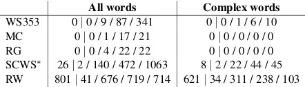
frequencies extracted from Wikipedia documents. It is interesting to observe that WS353, MC, RG contain very frequent words and have few complex words (only WS353 has).12_SCWS∗_{and RW have} a more diverse set of words in terms of frequencies and RW has the largest number of unknown and rare words, which makes it a challenging dataset.

All words Complex words

WS353 0|0 / 9 / 87 / 341 0|0 / 1 / 6 / 10 MC 0|0 / 1 / 17 / 21 0|0 / 0 / 0 / 0 RG 0|0 / 4 / 22 / 22 0|0 / 0 / 0 / 0 SCWS∗ _{26|2 / 140 / 472 / 1063 8|2 / 22 / 44 / 45}

RW 801|41 / 676 / 719 / 714 621|34 / 311 / 238 / 103

Table 4:Word distribution by frequencies– dis-tinct words in each dataset are grouped based on frequencies and counts are reported for the fol-lowing bins : unknown|[1, 100] / [101, 1000] / [1001, 10000] / [10001,∞). We report counts for all words in each dataset as well as complex ones.

5.1.1 Rare Word Dataset

As evidenced in Table 4, most existing word sim-ilarity datasets contain frequent words and few of them possesses enough rare or morphologically complex words that we could really attest the ex-pressiveness of our morphoRNN models. In fact, we believe a good embedding in general should be able to learn useful representations for not just fre-quent words but also rare ones. That motivates us to construct another dataset focusing on rare words to complement existing ones.

Our dataset construction proceeds in three stages: (1) select a list of rare words, (2) for each of the rare words, find another word (not neces-sarily rare) to form a pair, and (3) collect human judgments on how similar each pair is.

(5, 10] (10, 100] (100, 1000]

un- untracked unrolls undissolved unrehearsed unflagging unfavourable unprecedented unmarried uncomfortable

-al apocalyptical traversals bestowals acoustical extensional organismal directional diagonal spherical

-ment obtainment acquirement retrenchments discernment revetment rearrangements confinement establishment management

word1 untracked unflagging unprecedented apocalyptical organismal diagonal obtainment discernment confinement

word2 inaccessible constant new prophetic system line acquiring knowing restraint

Table 5:Rare words(top) –word1by affixes and frequencies and sampleword pairs(bottom).

Rare word selection: our choices of rare words (word1) are based on their frequencies – based on

five bins (5, 10], (10, 100], (100, 1000], (1000, 10000], and the affixes they possess. To create a diverse set of candidates, we randomly select 15 words for each configuration (a frequency bin, an affix). At the scale of Wikipedia, a word with frequency of 1-5 is most likely a junk word, and even restricted to words with frequencies above five, there are still many non-English words. To counter such problems, each word selected is re-quired to have a non-zero number of synsets in WordNet(Miller, 1995).

Table 5 (top) gives examples of rare words se-lected and organized by frequencies and affixes. It is interesting to find out that words likeobtainment andacquirement are extremely rare (not in tradi-tional dictionaries) but are perfectly understand-able. We also have less frequent words like revet-mentfrom French ororganismalfrom biology.

Pair construction: following (Huang et al., 2012), we create pairs with interesting relation-ships for each word1 as follow. First, a

Word-Net synset ofword1is randomly selected, and we

construct a set of candidates which connect to that synset through various relations, e.g., hypernyms, hyponyms, holonyms, meronyms, and attributes. Aword2is then randomly selected from these

can-didates, and the process is repeated another time to generate a total of two pairs for each word1.

Sample word pairs are given in Table 5 in which word2 includes mostly frequent words, implying

a balance of words in terms of frequencies in our dataset. We collected 3145 pairs after this stage

Human judgment: we use Amazon Mechani-cal Turk to collect 10 human similarity ratings on a scale of [0, 10] per word pair.13 _{Such procedure}

has been demonstrated by Snow et al. (2008) in replicating ratings for the MC dataset, achieving close inter-annotator agreement with expert raters. Since our pairs contain many rare words which are

13_{We restrict to only US-based workers with 95% approval} rate and ask for native speakers to rate 20 pairs per hit.

challenging even to native speakers, we ask raters to indicate for each pair if they do not know the first word, the second word, or both. We use such information to collect reliable ratings by either dis-card pairs which many people do not know or col-lect additional ratings to ensure we have 10 rat-ings per pair.14 _{As a result, only 2034 pairs are}

retained.

5.2 Results

We evaluate the quality of our morphoRNN em-beddings through the word similarity task dis-cussed previously. The Spearman’s rank correla-tion is used to gauge how well the relacorrela-tionship be-tween two variables, the similarity scores given by the NLMs and the human annotators, could be de-scribed using a monotonic function.

Detailed performance of the morphoRNN em-beddings trained from either the HSMN or the C&W embeddings are given in Table 7 for all datasets. We also report baseline results (rows HSMN, C&W) using these initial embed-dings alone, which interestingly reveals strengths and weaknesses of existing embeddings. While HSMN is good for datasets with frequent words (WS353, MC, and RG), its performances for those with more rare and complex words (SCWS∗ _and RW) are much inferior than those of C&W, and vice versa. Additionally, we consider two slightly more competitive baselines (rows +stem) based on the morphological segmentation of unknown words: instead of using a universal vector repre-senting all unknown words, we use vectors rep-resenting the stems of unknown words. These baselines yield slightly better performance for the SCWS∗_{and RW datasets while the trends we} men-tioned earlier remain the same.

Our first model, the context-insensitive mor-phoRNN (cimRNN), outperforms its correspond-ing baseline significantly over the rare word

Words C&W C&W + cimRNN C&W + csmRNN

commenting insisting insisted focusing hinted republishing accounting expounding commented comments criticizing comment commentary rant statement remark commentary rant statement remark rant commentary statement anecdote distinctness morphologies pesawat clefts modality indistinct tonality spatiality indistinct distinctiveness largeness uniqueness distinct different distinctive broader narrower different distinctive broader divergent divergent diverse distinctive homogeneous unaffected unnoticed dwarfed mitigated disaffected unconstrained uninhibited undesired unhindered unrestricted affected caused plagued impacted damaged disaffected unaffected mitigated disturbed complicated desired constrained reasoned unaffect ∅ affective affecting affectation unobserved affective affecting affectation restrictive affect exacerbate impacts characterize affects affectation exacerbate characterize decrease arise complicate exacerbate heartlessness ∅ fearlessness vindictiveness restlessness depersonalization terrorizes sympathizes heartless merciless sadistic callous mischievous merciless sadistic callous mischievous sadistic callous merciless hideous heart death skin pain brain life blood death skin pain brain life blood death brain blood skin lung mouth saudi-owned avatar mohajir kripalani fountainhead saudi-based somaliland al-jaber saudi-based syrian-controlled syrian-backed short-changed kindled waylaid endeared peopled conformal conformist unquestionable short-termism short-positions self-sustainable

Table 6:Nearest neighbors. We show morphologically related words and their closest words in different representations (“unaffect” is a pseudo-word;∅marks no results due to unknown words).

WS353 MC RG SCWS∗ _RW

HSMN 62.58 65.90 62.81 32.11 1.97 +stem 62.58 65.90 62.81 32.11 3.40 +cimRNN 62.81 65.90 62.81 32.97 14.85 +csmRNN 64.58 71.72 65.45 43.65 22.31

C&W 49.77 57.37 49.30 48.59 26.75 +stem 49.77 57.37 49.30 49.05 28.03 +cimRNN 51.76 57.37 49.30 47.00 33.24 +csmRNN 57.01 60.20 55.40 48.48 34.36

Table 7:Word similarity task– shown are Spear-man’s rank correlation coefficient (ρ ×100)

be-tween similarity scores assigned by neural lan-guage models and by human annotators. stem in-dicates baseline systems in which unknown words are represented by their stem vectors.cimRNNand csmRNNrefer to our context insensitive and sensi-tive morphological RNNs respecsensi-tively.

dataset. The performance is constant for MC and RG (with no complex words) and modestly im-proved for MC (with some complex words – see Table 4). This is expected since the cimRNN model only concerns about reconstructing the original embedding (while learning word struc-tures), and the new representation mostly differs at morphologically complex words. For SCWS∗_, the performance, however, decreases when train-ing with C&W, which perhaps is due to: (a) the baseline performance of C&W for SCWS∗_is com-petitive and (b) the model trades off between learn-ing syntactics (the word structure) and capturlearn-ing semantics, which requires context information.

On the other hand, the context-sensitive mor-phoRNN (csmRNN) consistently improves corre-lations over the cimRNN model for all datasets, demonstrating the effectiveness of using surround-ing contexts in learnsurround-ing both morphological

syn-tactics and semantics. It also outperforms the corresponding baselines by a good margin for all datasets (except for SCWS∗_{). This highlights the} fact that our method is reliable and potentially ap-plicable for other embeddings.

6 Analysis

To gain a deeper understanding of how our mor-phoRNN models have “moved” word vectors around, we look at nearest neighbors of sev-eral complex words given by various embed-dings, where cosine similarity is used as a dis-tance metric. Examples are shown in Table 6 for three representations: C&W and the context-insensitive/sensitive morphoRNN models trained on the C&W embedding.15

Syntactically, it is interesting to observe that the cimRNN model could well enforce structural agreement among related words. For example, it returnsV-ing as nearest neighbors for “comment-ing” and similarly, JJ-ness for “fearlessness”, an unknown word that C&W cannot handle. How-ever, for those cases, the nearest neighbors are badly unrelated.

On the semantic side, we notice that when structural agreement is not enforced, the cimRNN model tends to cluster words sharing the same stem together, e.g., rows with words of the form affect .16 _{This might be undesirable when we}

want to differentiate semantics of words sharing the same stem, e.g. “affected” and “unaffected”.

The csmRNN model seems to balance well be-tween the two extremes (syntactic and seman-tic) by taking into account contextual information

15_{Results of HSMN-related embeddings are not shown, but} similar trends follow.

when learning morphological structures. It returns neighbors of the same structureun edfor “unaf-fected”, but does not include any negation of “af-fected” in the top 10 results when “af“af-fected” is queried.17 _{Even better, the answers for}

“distinct-ness” have blended well both types of results.

7 Conclusion

This paper combines recursive neural networks (RNNs) and neural language models (NLMs) in a novel way to learn better word representa-tions. Each of these components contributes to the learned syntactic-semantic word vectors in a unique way. The RNN explicitly models the mor-phological structures of words, i.e., the syntactic information, to learn morphemic compositional-ity. This allows for better estimation of rare and complex words and a more principled way of han-dling unseen words, whose representations could be constructed from vectors of known morphemes. The NLMs, on the other hand, utilize surround-ing word contexts to provide further semantics to the learned morphemic representations. As a result, our context-sensitive morphoRNN em-beddings could significantly outperform existing embeddings on word similarity tasks for many datasets. Our analysis reveals that the model could blend well both the syntactic and semantic infor-mation in clustering related words. We have also made available a word similarity dataset focusing on rare words to complement existing ones which tend to include frequent words.

Lastly, as English is still considered limited in terms of morphology, our model could poten-tially yield even better performance when applied to other morphologically complex languages such as Finnish or Turkish, which we leave for future work. Also, even within English, we expect our model to be value to other domains, such as bio-NLP with complicated but logical taxonomy.

Acknowledgements

We thank the anonymous reviewers for their feed-back and Eric Huang for making his various pieces of code available to us as well as answering our questions on different datasets. Stanford Uni-versity gratefully acknowledges the support of the Defense Advanced Research Projects Agency (DARPA) Deep Exploration and Filtering of Text

17_{“disaffected” is ranked 5}th_{for the first query while}

“af-fecting” occurs at position 8 for the latter.

(DEFT) Program under Air Force Research Lab-oratory (AFRL) contract no. FA8750-13-2-0040 and the DARPA Broad Operational Language Translation (BOLT) program through IBM. Any opinions, findings, and conclusion or recommen-dations expressed in this material are those of the authors and do not necessarily reflect the view of the DARPA, AFRL, or the US government.

References

Andrei Alexandrescu and Katrin Kirchhoff. 2006. Factored neural language models. InNAACL.

Y. Bengio, R. Ducharme, P. Vincent, and C. Janvin. 2003. A neural probabilistic language model. Jour-nal of Machine Learning Research, 3:1137–1155.

Alexander Clark. 2003. Combining distributional and morphological information for part of speech induc-tion. InEACL.

R. Collobert and J. Weston. 2008. A unified archi-tecture for natural language processing: deep neural networks with multitask learning. InICML.

R. Collobert, J. Weston, L. Bottou, M. Karlen, K. Kavukcuoglu, and P. Kuksa. 2011. Natural lan-guage processing (almost) from scratch. Journal of Machine Learning Research, 12:2493–2537.

R. Collobert. 2011. Deep learning for efficient dis-criminative parsing. InAISTATS.

Mathias Creutz and Krista Lagus. 2007. Unsuper-vised models for morpheme segmentation and mor-phology learning. ACM Transactions on Speech and Language Processing, 4:3:1–3:34.

Lev Finkelstein, Evgeniy Gabrilovich, Yossi Matias, Ehud Rivlin, Zach Solan, Gadi Wolfman, and Ey-tan Ruppin. 2002. Placing search in context: the concept revisited. ACM Transactions on Informa-tion Systems, 20(1):116–131.

Michael Gasser and Chan-Do Lee. 1990. A short-term memory architecture for the learning of mor-phophonemic rules. InNIPS.

Michael Gasser. 1994. Acquiring receptive morphol-ogy: A connectionist model. InACL.

X. Glorot, A. Bordes, and Y. Bengio. 2011. Domain adaptation for large-scale sentiment classification: A deep learning approach. InICML.

E. H. Huang, R. Socher, C. D. Manning, and A. Y. Ng. 2012. Improving word representations via global context and multiple word prototypes. In Annual Meeting of the Association for Computational Lin-guistics (ACL).

Terry Koo, Xavier Carreras, and Michael Collins. 2008. Simple semi-supervised dependency parsing. InACL.

Angeliki Lazaridou, Marco Marelli, Roberto Zampar-elli, and Marco Baroni. 2013. Compositional-ly derived representations of morphologically complex words in distributional semantics. InACL.

Tomas Mikolov and Geoffrey Zweig. 2012. Context dependent recurrent neural network language model. InSLT.

Tomas Mikolov, Martin Karafi´at, Lukas Burget, Jan Cernock´y, and Sanjeev Khudanpur. 2010. Recur-rent neural network based language model. In IN-TERSPEECH.

Tomas Mikolov, Stefan Kombrink, Lukas Burget, Jan Cernock´y, and Sanjeev Khudanpur. 2011. Exten-sions of recurrent neural network language model. InICASSP.

Tomas Mikolov, Wen-tau Yih, and Geoffrey Zweig. 2013. Linguistic regularities in continuous space word representations. InNAACL-HLT.

George A. Miller and Walter G. Charles. 1991. Con-textual correlates of semantic similarity. Language and Cognitive Processes, 6(1):1–28.

G.A. Miller. 1995. WordNet: A Lexical Database for English. Communications of the ACM.

Andriy Mnih and Geoffrey Hinton. 2007. Three new graphical models for statistical language modelling. InICML.

Andriy Mnih and Geoffrey Hinton. 2009. A scalable hierarchical distributed language model. InNIPS.

Frederic Morin. 2005. Hierarchical probabilistic neu-ral network language model. AIstats’05. In AIS-TATS.

K. Plunkett and V. Marchman. 1991. U-shaped learn-ing and frequency effects in a multi-layered percep-tron: implications for child language acquisition. Cognition, 38(1):43–102.

Lev Ratinov and Dan Roth. 2009. Design challenges and misconceptions in named entity recognition. In CoNLL.

Nathan D. Ratliff, J. Andrew Bagnell, and Martin A. Zinkevich. 2007. Online subgradient methods for structured prediction.

Joseph Reisinger and Raymond J. Mooney. 2010. Multi-prototype vector-space models of word mean-ing. InNAACL.

Herbert Rubenstein and John B. Goodenough. 1965. Contextual correlates of synonymy. Communica-tions of the ACM, 8(10):627–633.

David E. Rumelhart and James L. McClelland. 1986. On learning the past tenses of English verbs. In J. L. McClelland, D. E. Rumelhart, and PDP Research Group, editors,Parallel Distributed Processing. Vol-ume 2: Psychological and Biological Models, pages 216–271. MIT Press.

Cyrus Shaoul and Chris Westbury. 2010. The West-bury lab wikipedia corpus. Edmonton, AB: Univer-sity of Alberta.

Noah A. Smith and Jason Eisner. 2005. Contrastive estimation: training log-linear models on unlabeled data. InACL.

Rion Snow, Brendan O’Connor, Daniel Jurafsky, and Andrew Y. Ng. 2008. Cheap and fast—but is it good?: Evaluating non-expert annotations for nat-ural language tasks. InEMNLP.

Richard Socher, Christopher Manning, and Andrew Ng. 2010. Learning continuous phrase represen-tations and syntactic parsing with recursive neural networks. InNIPS*2010 Workshop on Deep Learn-ing and Unsupervised Feature LearnLearn-ing.

R. Socher, E. H. Huang, J. Pennington, A. Y. Ng, and C. D. Manning. 2011a. Dynamic pooling and un-folding recursive autoencoders for paraphrase detec-tion. InNIPS.

R. Socher, Cliff C. Lin, A. Y. Ng, and C. D. Manning. 2011b. Parsing natural scenes and natural language with recursive neural networks. InICML.

R. Socher, J. Pennington, E. H. Huang, A. Y. Ng, and C. D. Manning. 2011c. Semi-supervised recursive autoencoders for predicting sentiment distributions. InEMNLP.

R. Socher, B. Huval, C. D. Manning, and A. Y. Ng. 2012. Semantic compositionality through recursive matrix-vector spaces. InEMNLP.