Abstract— Subsea plumes are caused by uncontrolled release of fluids from a well during drilling or leakages from risers or pipelines. Subsea plumes can cause water pollution, fire and instability of rigs and floating vessels. The consequences of subsea plume formation can be catastrophic with severe financial, health and safety implications. In this paper, an existing numerical model for subsea multiphase single plume based on the Eularian integral approach is modified to suit moderate water depth conditions. The numerical equations are programmed using Matlab 7.6.0. A case study of 500m water depth is used to demonstrate the practical application of the model. This predicts more accurately the radius and velocity of plumes in comparison to conventional approximate solutions. It shows that the momentum amplification factor has a significant effect on plume behaviour. The model is a robust risk analysis tool which accurately predicts the size, rate of spread and extent of plumes in order to effectively manage its potential consequences.
Index Terms—Subsea, Plume, Modelling, Eulerian integral approach
.
I. INTRODUCTION
Subsea release of liquids and/or gases is one of the major challenges in the offshore oil and gas sector. The releases are caused by blowouts and leakages from risers or pipelines. These often result in formation of plumes;buoyantliquid or gases released in seawater [1]. Plumes are classified as single or multiphase [2] and are of different densities compared to the surrounding seawater. The variation in densities often result in slippage between the phases [3]. The released gases interact with the surrounding seawater to form bubbles dispersed within the plume trajectory.
Subsea plumes can cause water pollution, fire and
Manuscript received November 6, 2009. (Write the date on which you submitted your paper for review.)
Abass Abubakr-Bibilazu is with the Energy Centre, School of Engineering, Robert Gordon University, Schoolhill Aberdeen AB10 1FR,U.K (a.abu-bakr-bibilazu@ rgu.ac.uk).
Jesse A Andrawus is a lecturer at the Energy Centre of the School of Engineering, Robert Gordon University, Schoolhill B10 1FR, Aberdeen, U.K (phone: 0044 1224 262304 ;Fax: 0044 1224 262444 e-mail: [email protected]).
Ebenezer Adom is a Lecturer at the School of Engineering, Robert Gordon University, Schoolhill, Aberdeen, AB10 1FR, U.K (e-mail: [email protected]).
John A Steel, is a Professor at The Robert Gordon University, Schoohill, Aberdeen,AB10 1FR(email:[email protected])
*Tuoyo Brikinns, Saipem UK Ltd, Sonsub Division Tern Place Denmore Road, Bridge of Don, Aberdeen AB23 8JX, U.K
instability of rigs and floating vessels due to loss of buoyancy flux. These can be catastrophic with massive financial, health and safety consequences. Thus, there is a need to accurately predict the movement of released hydrocarbons in a column of seawater in order to mitigate its potential consequences.
The plume modelling software packages do not take into account the effect of gas compressibility and hydrate formation. The software packages use shallow water considerations for modelling plume behaviour in moderate water depth. Thus, predictions of plume behaviour and surface spread-out are over or under estimated. In this paper, an existing numerical model for subsea multiphase single plume is modified to suit moderate water depths based on an Eularian Integral Approach.
II. PLUME DEVELOPMENT ZONES
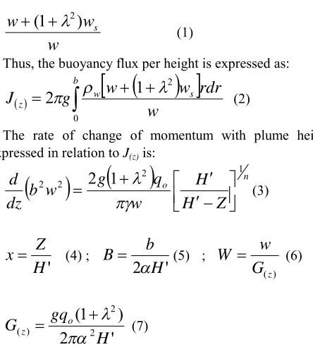
Plumes are generally cone shaped with three development zones;flow establishment(jet),established flow(pure plume) andsurface flow[4].
The first plume field experiment carried out by Rye et al [5], identified the phenomenon of plume diameter decreasing beyond a certain height as surface water is approached. There was no evidence of plume regeneration. The study was not conclusive thus recommended further investigations.
III. NUMERICAL PLUME MODELLLING Previous studies in the area of subsea plumes has largely been focused on single plume models ([5],[6];[7]) and double plume models ([2];[8];[9];). However, the double plume model seldom occurs [6]. Fannelop and Sjoen [6] developed a numerical plume model for shallow water based on the Eulerian Integral concept.
The development of numerical integral plume models has evolved from Eulerian concepts ([10]; [11]) to Lagrangian concepts ([12]; [13]; [14]). In both concepts, a control volume is assumed, that is, Eulerian assumes afixedcontrol volume whilst Lagrangian assumes a variable volume which traces the path of the plume trajectory. The Lagrangian concept [12] is an improvement on the Eulerian concept taking into account the effects of cross currents, non-ideal gas behaviour, dissolution of gas from bubbles and hydrates formation. Rye [15] modified Fannelop and Sjoen’s [6] approach and included oil dissolution from plume to ambient water and gas expansion. It is worth noting however that the move from an Eulerian to Lagrangian concept was as a result of increases in gas dissolution and hydrate formation in deep water [14]. However, if hydrates do not form it would be valid to apply
Numerical Modelling of Subsea Multiphase
Plumes: An Eularian Integral Approach
the Eulerian Integral approach.
Modelling Equations & Data Requirements
The governing plume equations are based on conservation of volume flux, mass flux, momentum and buoyancy flux. Fannelop and Sjoen [6] demonstrated mathematically that the density difference between the water density ( ) and plume density in their formulations will differ from that by Ditmars and Cederwall [16] by a factor
w
w
w
(
1
)
s2
(1)
Thus, the buoyancy flux per height is expressed as:
b s w zw
rdr
w
w
g
J
0 21
2
(2)The rate of change of momentum with plume height expressed in relation toJ(z)is:
no
Z
H
H
w
q
g
w
b
dz
d
2 22
1
2 1
(3)'
H
Z
x
(4) ;'
2
H
b
B
(5) ;) (z
G
w
W
(6)'
2
)
1
(
2 2 ) (H
gq
G
o z
(7)Note, the Fannelop and Sjoen [6] model did not include momentum amplification factor (γ) as suggested later by Milgram [17].γaccounts for the variation in plume velocity from the jet zone to the pure plume zone. In this paper,γis accounted for as shown in equation 3.
Fannelop and Sjoen’s [6] formulations of plume equations were based only on ideal gas behaviour (shown in equation 3). In this paper, the numerical model is extended to account for real gas behaviour. The gas void fraction could further be expressed to account for gas compressibility effects as:
2
2 2 21
(
1
b
w
w
T
m
k
Z
H
T
m
k
H
q
S
s n o go o z g z oz
(8)Thus, eq. (3) becomes
n
o go o Z z g z o
T
m
k
Z
H
T
m
k
H
w
q
g
w
b
dz
d
2 () () ( )2
2
2
1
(9)
The test conditions used in modelling the plume behaviour are shown in Table 1.
TABLE1: PLUMEMODELLINGDATA
CONDITIONS CASE STUDY
Depth of Water (H) 500m
Leakage Diameter (D) 0.08m
Pipeline Temperature (T) 290 K Pipeline Pressure (P) 500N/m2 Entrainment Coefficient (α) 0.165 Momentum Amplification
Factor (γ)
1.3
Height of Pipeline above seabed (h)
1m
Gas Composition Methane
Drag Coefficient 0.65
Gas Specific Heat Ratio (n) 1.1
IV. ANALYSES AND DISCUSSION
The non-dimensional height
(
x
)
obtained from simulation of the plume model ranged between 0.0040 and 0.9604 (see table 2). The corresponding plume height (Z) ranged between 0.2089m and 488.8489m. A cone-shaped angle approximately 22.10 was used in the modelling as this compares to reported cone angles ([15]). However, fountain formation ([6]; [18];[19]) was not observed within this range. This implies that the height at which the model terminates is still within the steady state zone (Zone of Established Flow). The phenomenon of a fountain is a distinct feature seen at the surface of water as a result of plume rising above the water surface. The model is programmed to calculatex
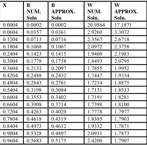
in steps of 0.06. Reduction in the step height reduces the interval between the heights. Thus, the height at which the model terminates would be closer to the end ofzone of established flow. [image:2.595.55.277.176.422.2] [image:2.595.57.273.296.422.2]parameters. The numerical solution indicated that W drops sharply as the plume rises from 20.9564 to 2.9260, signifying the transition from the jet zone to the pure plume zone. In the pure plume zone, W remains fairly constant and tends to a value of 1.7131. Subsequently, as the plume approaches surface,wincreases slowly to a value of 2.4200.
Fig.1a: Ideal Plume Shape Fig.1b Variation in Plume Shape as Surfaceis (Cone-Shape)
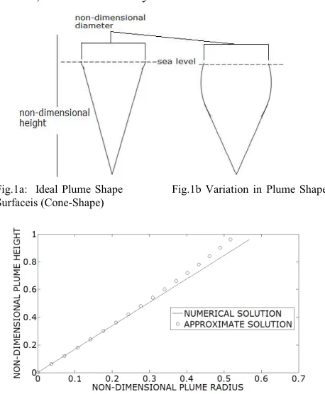
Fig. 2: Non-Dimensional Plume Height and Radii for Numerical and
[image:3.595.55.271.431.547.2]Approximate Solutions
Fig. 3: Non-Dimensional Plume Height and Velocity for Numerical and Approximate Solutions.
The approximate solution curve for wis asymptotic to a low limiting value of 1.7871 asxincreases whilst that of the numerical solution is concave-shaped (see fig.3). At an x value of about 0.8 to water surface, the numerical solution deviate from the approximate solution by about 9% to 43% for values of W. This is reflected in the shapes of the approximate and numerical solutions (fig. 3). The numerical results for plume radius and velocity ranged from 0.04m to 95.4646m and 10.1398m/s to 1.1709m/s respectively. For the approximate solution, the results were slightly different with the b and w ranging from 0.0414m to 86.9278m and 8.3160m/s to 0.8664 respectively.
The Densimetric Froude Number (DFN) concept [20] is used to establish the initial conditions. The starting plume height (z) andxare 0.4m and 0.0025 respectively. The Virtual Source Point ([17] ,[21];) concept compared to DFN clearly over-estimates the starting x for numerical integration by
about twice the values as would Fannelop and Sjoen’s [6] model. Fannelop and Sjoen’s [6]; Freidl [18], who claimed the x may approximated to plume source. However, this appears to be invalid! Although the initial value ofxis very close to the plume source, it would be improper to approximate this height to plume source as this corresponds to significant W value velocities which cannot be ignored. Ignoring thisWvalue would affect considerably the numerical results for initialWvalue;subsequentWvalues as plume rises and the rise time used in risk analysis.
Effect of momentum amplification factor (γ) on plume velocity (w)
Milgram [17] was the first to include the effect ofγ into
integral plume models.The introduction of γ reduces all the values of w as values x changes by a factor of (1/γ). The sensitivity of plume velocity as momentum amplification factor varies is shown in Fig.4 and Fig.5. The numerical solution attains a deviation of 3% for w when γ is varied between 1 and 1.3. On the other hand, the approximate solution shows a deviation of 0.0036% when γ is varied between 1 and 1.3. Overall, increasingγ will result in lower values ofwand vice-versa. The effect of varying γ(between 1.0. and 1.3) on approximate solutions are negligible (0.0036% deviation) but of significant importance in numerical solution (3% deviation). It is important to obtain accurate estimation ofγ from field and experimental data in order to use the numerical solution.
[image:3.595.313.548.444.594.2]Fig. 5: Effect of Momentum Amplification Factor on Plume Height and
Centre-line Velocity based on Approximate Solution
Effect of gas compressibility
Gases obey the ideal gas equation for which case, the gas compressibility factor is taken as unity. However, when the gas compressibility factor changes to values greater than unity or less than unity, there is the need to modify the ideal gas equation by introducing the gas compressibility factor (k(z)).
The gas compressibility factor varied from 1 to 0.95 for water depth 0-210m and 0.95 to 0.90 for water depth 210-400m. The closer the plume is to the water surface, the lower the gas compressibility factor. A logical explanation is the influence of hydrostatic pressure. This becomes greater as the depth of water increases. Thus, the higher the hydrostatic pressure, the greater the compressibility effect (less than unity) on gases closer to the plume source. Thus k(z)deviates from unity by 3.7% for 500m water depth. Figure 6 shows the changes in gas compressibility factors as the depth of water changes.
0.86 0.88 0.9 0.92 0.94 0.96 0.98 1 1.02
0 100 200 300 400 500 600
G
A
S
CO
M
PR
ES
SI
B
LI
TY
FA
CT
O
R
DEPTH OF SEAWATER (m)
[image:4.595.55.294.51.201.2]IDEAL BEHAVIOUR OF METHANE GAS NON-IDEAL BEHAVIOUR OF METHANE GAS
Fig. 6: Plot of Ideal and Non-Ideal Behaviour of Methane against Seawater Depth
[image:4.595.304.550.86.329.2]At distances closer to the plume source, the number of moles of gas trapped in a bubble would be reduced by a factor equal to thek(z)for cases wherek(z)<1. Thus, the concentration of a particular kind of gas present would subsequently reduce.
TABLE 2: Results of Numerical and Approximate Solutions for Non-dimension plume velocity and radius
X B
NUM. Soln
B APPROX. Soln
W NUM. Soln.
W APPROX. Soln. 0.0004 0.0002 0.0002 20.9564 17.1871 0.0604 0.0357 0.0361 2.9260 3.3072 0.1204 0.0713 0.0716 2.3567 2.6718 0.1804 0.1068 0.1067 2.0972 2.3758 0.2404 0.1423 0.1415 1.9460 2.1983 0.3004 0.1778 0.1758 1.8493 2.0795 0.3604 0.2133 0.2097 1.7855 1.9952 0.4204 0.2488 0.2432 1.7447 1.9334 0.4804 0.2843 0.2761 1.7214 1.8875 0.5404 0.3198 0.3084 1.7131 1.8533 0.6004 0.3553 0.3402 1.7191 1.8281 0.6604 0.3908 0.3714 1.7398 1.8100 0.7204 0.4263 0.4020 1.7778 1.7977 0.7804 0.4618 0.4319 1.8385 1.7903 0.8404 0.4973 0.4612 1.9332 1.7871 0.9004 0.5328 0.4897 2.0911 1.7873 0.9604 0.5683 0.5175 2.4200 1.7907
V. CONCLUSION & FUTURE WORK
An existing numerical shallow water plume model [6] was modified to suit moderate water depth (500m) conditions. The numerical model was based on an Eulerian Integral Approach. The model was applied to a gas pipeline leakage case study to demonstrate its practical application with the results compared with approximate solutions. The numerical model exhibited 3% and 8% deviation respectively from the approximate solution for values ofbandw. The approximate solution is observed to under-estimate the plume radius beyond 50% of the plume height when compared to the numerical solution. The effect of varying γ(between 1.0. and 1.3) on approximate solutions are negligible (0.0036% deviation) while it is significantly important in the numerical solution (3% deviation).
The reduction in cone angle observed by Fannelop and Sjoen [6]; Rye et al [5] accounts for the reduction in plume radii. Although not stated by Fannelop and Sjoen [6]; Rye et al [5] in their research, the phenomenon of reducing cone angle and plume width maybe as a result of water turbulence as water surface is approached. However, the use of a constant cone angle throughout the plume development fits the cone-shape the plume is alluded to have in cases where turbulence is neglected as seawater surface is approached. Thus, cone angles reducing as the water surface is approached is not observed in this paper. It is further observed that this turbulence is significant only after 50% of the non-dimensional height.
[image:4.595.59.295.470.632.2]VI. NOMENCLATURE b plume radius (m)
B non-dimensional plume radius g acceleration due to gravity (m/s2) G(Z) velocity parameter (m/s) H/water depth above pipeline (m) H total depth of water (m)
H0 height of pipeline above seabed (m)
J(z) buoyancy flux/plume height along centre -line (kg/s2) kogas compressibility factor at plume source
k(z) gas compressibility factor along plume centre-line mg mass flux of gas (kg/s)
mgo mass flux of gas at plume source(kg/s)
mg(z) mass flux of gas along plume centre-line (kg/s) n polytropic index
q(z) gas flux along the plume centre-line(m3/s) qo gas flux at plume centre-line (m3/s) r r- direction
S(z) Gas void fraction along plume centre-line To temperature at plume source (K)
T(z) temperature along plume centre-line(K) w plume velocity along centre-line
W non-dimensional plume velocity Z Plume height (m)
x non-dimensional plume height
α .entrainment coefficient.(dimensionless)
λ Schmidt number
γ momentum amplification factor
REFERENCES
[1] A. Chow, Effects of Buoyancy Source Composition on Multiphase Plume Behaviour in Stratification. . MIT, 2004.
[2] S. A. Socolofsky and E. E. Adams, Liquid Volume Fluxes in Stratified Multiphase Plumes, Journal of Hydraulic Engineering., Vol.129 11 (2003). [3] K. Cederwall and J. D. Ditmars, "Analysis of
Air-Bubble Plumes.," W. M. Keck Laboratory of Hydraulics and Water Resources, Division of Engineering and Applied Science, California Institute of Technology, Pasadena., 1970.
[4] S. L. R. E. Research, "Fate and Behaviour of Deepwater Subsea Oil Well Blowouts in The Gulf of Mexico.," 1997.
[5] H. Rye, Subsurface Blowouts: Results from Field Experiments, Spill Science and Technology Bulletin, 4 (1997), 239 – 256. .
[6] T. K. Fannelop and K. Sjoen, Hydrodynamics of Underwater blowouts, Norwegian Maritime Research 4 (1980), 17 -33.
[7] O. Johanssen, 2000. . , Deep Blow – A Lagrangian Plume Model for Deep Water Blowouts, Spill Science and Technology Bulletin,, 6:2 (2000), 103-111.
[8] T. J. Mcdougall, Bubble Plumes in Stratified Environments., Journal of Fluid Mechanics, , 14 (1978), 189 - 212.
[9] T. Asaeda and J. Imberger, Structure of Bubble Plumes in Linearly Stratified Environments, Journal of Fluid Mechanics. , 249 (1993), 35-57.
[10] E. Hirst, Buoyant Jets with Three Dimensional Trajectories, Journal of the Hydraulics Division, 98 11 (1972), 1999 – 2014.
[11] V. H. Chu and J. H. W. Lee, General Integral Formulation of Turbulent Buoyant Jets in Cross-flow, Journal of Hydraulic Engineering, 122 (1996), 27 – 34.
[12] J. H. W. Lee and V. Cheung, Generalized Lagrangian Model for Buoyant Jets in Current, Journal of Environmental Engineering, , 115:6 (1990), 1085 – 1105. .
[13] W. E. Frick, D. J. Baumgartner, and C. G. Fox, Improved Prediction of Bending Plumes, Journal of Hydraulic Research,, 32:6 (1994), 935 – 950. [14] O. Johansen, Development and Verification of
Deepwater Blowout Models, Marine Pollution Bulletin, 47 (2003), 360 – 368. .
[15] H. Rye, Model for Calculation of Underwater Blowout Plume, Proc. 17th ARCTIC Marine Oil Spill Programme (AMOP), 1994), 849-865. [16] J. D. Ditmars and K. Cederwall Analysis of
air-bubble plumes, Proc. Coastal Engng. , 1974), 2209–2226.
[17] J. H. Milgram, Mean Flow in Round Bubble Plumes, Journal of Fluid Mechanics. , 133 (1983), 345 - 376. [18] M. J. Friedl, Bubble Plumes and Their Interaction with Surface Water, Swiss Federal Institute of Technology., 1998.
[19] M. J. Friedl and T. K. Fannelop, Bubble Plumes and their Interaction with The Water Surface, Applied Ocean Research, 22 (2000), 199-128.
[20] A. Wuest, Bubble Plume Modelling for Lake Restoration. , Water Resources Research, 28:12 (1992), 3235-3250.