ConStance: Modeling Annotation Contexts to Improve Stance
Classification
Kenneth Joseph1 Lisa Friedland1 Will Hobbs1 David Lazer1 Oren Tsur1,2
{k.joseph, l.friedland, w.hobbs}@northeastern.edu [email protected],[email protected]
1Network Science Institute 2Software and Information Systems Engineering
Northeastern University Ben Gurion University of the Negev
Abstract
Manual annotations are a prerequisite for many applications of machine learning. However, weaknesses in the annotation process itself are easy to overlook. In par-ticular, scholars often choose what infor-mation to give to annotators without ex-amining these decisions empirically. For subjective tasks such as sentiment analy-sis, sarcasm, and stance detection, such choices can impact results. Here, for the task of political stance detection on Twit-ter, we show that providing too little con-text can result in noisy and uncertain an-notations, whereas providing too strong a context may cause it to outweigh other signals. To characterize and reduce these biases, we develop ConStance, a gen-eral model for reasoning about annotations across information conditions. Given con-flicting labels produced by multiple an-notators seeing the same instances with different contexts, ConStance simultane-ously estimates gold standard labels and also learns a classifier for new instances. We show that the classifier learned by ConStance outperforms a variety of base-lines at predicting political stance, while the model’s interpretable parameters shed light on the effects of each context.
1 Introduction
When annotators are asked for objective judg-ments about a text (e.g., POS tags), the broader context in which the text is situated is often ir-relevant. However, many NLP tasks focus on in-ference of factors beyond words and syntax. For example, the present work addresses the task of detecting political stance on Twitter. We ask
an-notators to determine whether a given Twitter user supports Donald Trump or Hillary Clinton. How-ever, inferring something about auserfrom a sin-gle tweet that she writes may prove difficult. Prior work on stance has relied on annotations collected this way (Mohammad et al.,2016b), but individual tweets do not always contain clear indicators.
One solution to this issue is to supply the anno-tator with more information about the user. For ex-ample, for the similar task of classifying a Twitter user’s political affiliation,Cohen and Ruths(2013) display the user’s last 10 tweets. Nguyen et al.
(2013), studying gender and age, ask annotators to label users by leveraging all information available in their profile. Thus, researchers have provided a range of contexts (or more broadly, information conditions) to annotators in an attempt to balance annotators’ exposure to the data needed for accu-racy with reasonable costs in terms of time, money and cognitive load.
However, while scholars routinely make such decisions about what information to show anno-tators, they rarely examine how such decisions ac-tually impact annotations. The first contribution of this paper (Section 3) is to show that, at least for political stance detection on Twitter, displaying different kinds of context to annotators yields sig-nificantly different annotationsfor the same user. As a result of these discrepancies, the accuracy of models trained on these annotations varies widely. While it is possible one could select a “best” context for a given task, our results suggest that doing so a priori is difficult and that, moreover, different contexts provide complementary infor-mation. What we would prefer, instead, is a model that learnshow contexts affect annotators andcombinesannotations from multiple contexts to create gold standard labels.
Fortunately, prior work suggests mechanisms for such a model. Typically in annotation tasks,
each item is judged by several annotators, and the resulting labels are aggregated, usually by major-ity vote, to create a gold standard. As an alterna-tive to majority vote,Raykar et al.(2010) develop an elegant probabilistic approach for learning to aggregate labels produced by annotators of vary-ing quality. Their model jointly estimates gold standard labels (in the form of probability scores), infers annotator error rates, and learns a classifier for use on out-of-sample data.
Our second contribution (Section 4) is an ex-tension of Raykar et al.’s model to handle labels not only created by annotators of varying quality, but also produced underinformation conditionsof varying quality. We call this model ConStance1.
LikeRaykar et al.(2010), who find that even quality annotators are useful, we find that low-quality contexts can be useful. Specifically, we find that the classifier produced from our model performs better than any classifier trained by ma-jority vote from the same labels. Furthermore, the model provides an unsupervised method for com-paring the information conditions by examining their respective error patterns.
Intuitively, ConStance performs a role analo-gous to boosting for annotations: for an arbitrary task, it permits collection of labels that capture dif-ferent aspects of the instances at hand, then com-bines them automatically to determine which are more reliable and to produce a classifier that takes all this into account.
2 Annotating Political Stance 2.1 Political Stance Detection
Stance detection is defined as the task of determin-ing whether an individual is in favor of, against, or neutral towards a target concept based on the content they have generated (Mohammad et al.,
2016b). It is related to but distinct from sentiment analysis: a given document can have negative sen-timent but a positive stance towards a particular target, or vice versa. Further, for stance detec-tion, the target need not be explicitly mentioned. These points are best illustrated via example: the tweet “I hope that the Democrats get destroyed in this election!” has a negative sentiment (towards Democrats), and (therefore, most likely) implies a
1 Replication materials for this work, including code
for ConStance, are available athttps://github.com/ kennyjoseph/constance. The paper’s Supplementary Material can also be accessed there.
positive stance towards Donald Trump.
As a case study for how context impacts an-notations, we focus on political stance detection on Twitter—specifically, determining stance to-wards Hillary Clinton and Donald Trump during the 2016 U.S. election season. This task illus-trates the challenges of annotation, since individ-ual tweets are often ambiguous with respect to stance, contexts on Twitter are inherently frac-tured, and differing contexts can make annotators lean in different directions.
Note that a user’s stance, as we use the term in this paper, is a latent (and stable) property of the user. However, short of interviewing the user, we can never be completely certain of her stance. As such, the examples here and evaluations later rely on the authors’ best estimates of stance, using all available information.
A user’s tweets, in turn, may or may not reveal her stance. This means that, by our definitions, an annotator might accurately perceive no stance in a tweet, yet have their annotation be considered incorrect with respect to the user’s true stance. We would consider this case an annotator error caused by lack of context.
As examples of the task, consider annotating the following three tweets: (i) “crooked Hillary - #lock-HerUp,” (ii) “Lester thinks he can control the crowd when he can’t even keep Trump on topic lmao,” and (iii) “ Set-tling in for #debatenight Hoping to hear an adult conversa-tion.” In the case of (i), a passing familiarity with
American politics gives us high confidence that the author is pro-Trump. The tweets in (ii) and (iii) are more ambiguous, but the authors’ stances become clearer with access to varying forms of context. For (ii), a Pepe the frog image (a sym-bol used by the American alt-right movement) in the user profile reveals that the user is probably a Trump supporter. Similarly, for (iii), a profile description that reads “Stereotypical Iowan who enjoys Hillary Clinton, progressive politics. Chair of CYDIWomen. Previously @HillaryForIA and @NARAL.” suggests
sup-port for Clinton and distaste for Trump.
deter-mine the stance of a user using data from one par-ticular time window.
2.2 Data
We collected tweets during the general election season (7/29/2016–11/7/2016) from over 40,000 Twitter users we had previously matched to voter registration records. Matching Twitter users to voter registrations (using methods similar to Bar-ber´a, 2016;Hobbs et al.,2017) helps ensure that the accounts we study are controlled by humans, and it supplies additional demographic variables: gender, race and party registered with.
We identified as a political tweet any tweet that mentioned the official handle for Donald Trump (@realDonaldTrump) or Hillary Clinton (@HillaryClinton), or that contained one or more of the following terms or hashtags: Hillary, Clin-ton, Trump, Donald, #maga, #imwithher, #de-batenight, #election2016, #electionnight. We re-moved all reply tweets, quote tweets and tweets that directly retweeted the candidates. Finally, we kept only those users who posted at least three po-litical tweets.
From these users, we sampled 562 political tweets for crowd-sourced stance annotation, se-lecting at most one tweet per user. These tweets were all sampled from users who were registered Democrats or Republicans. Half the tweets were paired with Hillary Clinton as the target, the other half with Donald Trump. We also sampled and set aside an additional 250 + 318 tweet/target pairs to use as development and validation data, respec-tively (see Section2.5).
2.3 Annotation Task
We used Amazon Mechanical Turk (AMT) for an-notation. Annotators were presented a triplet of
{tweet, target, context} and were asked to make their decisions on a 5-point Likert scale, ranging from “Definitely Opposes [target]” to “Definitely Supports [target]”. Both prior work (Mohammad et al.,2016b) and our pilot studies suggested con-fusion between options for a tweet’s irrelevance towards a target and the tweet’s neutrality towards the target, so we used the center of the scale for both options. For this paper, we use a narrower three-point scale formed by merging the “Defi-nitely” and “Probably” options.
Further, while tweets were annotated with re-spect to different targets, we combine all anno-tations into a single task by assuming that
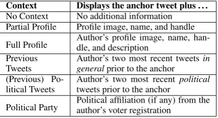
“anti-Context Displays the anchor tweet plus . . .
No Context No additional information Partial Profile Profile image, name, and handle Full Profile Author’s profile image, name, han-dle, and description Previous
Tweets Author’s two most recent tweetsgeneralprior to the anchor in (Previous)
[image:3.595.311.524.62.177.2]Po-litical Tweets Author’s two most recenttweets prior to the anchor political Political Party Political affiliation (if any) from theauthor’s voter registration
Table 1: Descriptions of the six contexts (informa-tion condi(informa-tions) presented to the annotators.
Trump” means “pro-Clinton”, and vice-versa. This assumption seems reasonable given that the voting population was strongly polarized during the general (post-primary) election season, and it doubles the amount of data we can use to train the models. Thus, throughout this work the labels we use are taken from the set{“Support Trump / Oppose Clinton”=−1, “Neutral / I don’t know” = 0, “Oppose Trump / Support Clinton”= 1}.
2.4 Contexts Studied
Each of the 562 “anchor” tweets was annotated under six differentcontexts(also referred to as in-formation conditions) described in Table 1. (The Supplementary Material provides visual examples of each.) We collected at least three annotations for each tweet/condition pair. Every AMT worker was shown 40 different tweets, one by one, ran-domly distributed across contexts. Two additional artificial tweets were used to control for task com-petency.
We selected the conditions in Table1based on two factors. First, we included conditions that var-ied in how much we expected them to impact an-notations. For example, we expected the partial profile information to have a relatively small ef-fect, and political party a larger one. Second, we restricted our options to sets of information that we believed would minimally impact task comple-tion times. We confirmed this empirically by re-gressing the (logged) time to completion for each annotator on the number of tweets she saw for each context, finding no significant effects from any context.
2.5 Gold Standard Labels
characterize for tasks as subjective as stance de-tection or sentiment analysis (Passonneau and Car-penter, 2014;DiMaggio, 2015). In light of this, we constructed our own labels, using all available information about users, and we use them as an approximation of ground truth.
We constructed these labels in order to evaluate downstream classification performance, and they cover a set of users not shown to the AMT work-ers. Given our resource constraints and the numer-ous (at least 18), often conflicting labels already available for tweets shown to AMT workers, we did not create definitive labels for that set.
To create these “gold standard” (GS) labels, we considered all information found on the user’s Twitter timeline, including everything AMT an-notators could see, plus friend/following relation-ships, all of their previous tweets, demographics from the voter file, etc. Anecdotally, we found cer-tain cases time-consuming to investigate, which argues for continuing to limit how much informa-tion we ask annotators to consider. All gold stan-dard labels were agreed upon by at least two au-thors, who first labeled the data independently and then came together to discuss disagreements.
Our GS set consists of 318 users (with their as-sociated anchor tweets). Each user is assigned a label from the tertiary Trump/Neutral/Clinton scale. Another 250 manually labeled accounts were used for model development but are not part of reported results. The GS is approximately equally divided among registered Democrats, reg-istered Republicans, and people not regreg-istered with either party; the last category includes self-declared Independents and voters not affiliated with any party. We include this third set in order to ensure the models generalize beyond registered Democrats and Republicans.
3 Annotation Quality For Individual Contexts
In this section, we examine how annotator agree-ment varies depending on the context in which the labels were obtained, and how classifiers trained on majority-vote labels from each individual con-text, as well as on labels from all contexts com-bined, perform on the GS. First, we introduce the classifier and features used for the latter task, then discuss results for agreement and classifier perfor-mance.
3.1 Classifier, Labels, Features, & Evaluation
For each of the six contexts separately, we con-struct labels with which to train a classifier. Train-ing labels are constructed usTrain-ing majority vote; we also tried weighting the training instances to match the distribution of labels, but it did not perform as well. We also construct a seventh set of labels us-ing all annotations from all conditions. We then train a classifier on each set of labels. We use Random Forest models, as they outperformed reg-ularized logistic regression and SVMs with linear kernels on the development set. Note that the only difference among the models in this section is the
labelsthey aretrainedon.
The feature set used, shown in Table2, is meant as a straightforward representation of the informa-tion seen by annotators; parts of it followEbrahimi et al.(2016). We construct three types of features for each tweet: text, sentiment and user features. For text features, we collapse the anchor tweet plus all additional textual context seen by any an-notator into a single string, then compute vari-ous n-grams from it. For sentiment, we compute various scores from the anchor tweet alone. For user features, we include the user’s race and gen-der, which annotators might have learned from the user’s profile picture. Note that because we want models to generalize beyond registered Democrats or Republicans, wedo notinclude a feature for po-litical party.
Classifier performance on the GS is measured, following prior work (Mohammad et al., 2016a;
Ebrahimi et al., 2016), on the average of the F1 scores on the two classes of interest (“Clinton” and “Trump”). Additionally, we report the aver-age log-loss (the negative log-likelihood, accord-ing to the classifier, of the true label). Log-loss and F1 can be seen as complementary measures: whereas F1 evaluates the quality of the ranking of test instances, log-loss evaluates the quality of their individual probability estimates. To compute the probability estimate from a Random Forest, we compute mean class probabilities across all trees.
Category Data Source Feature Representation
Text Anchor tweet,
previous (political) tweets, profile description
Character n-grams (n∈[3,5]), word n-grams (n∈[1,3]).
Preprocessing: only use tokens appearing≥10times, apply tf-idf weighting.
[image:5.595.69.530.61.137.2]Sentiment Anchor tweet VADER score (Dictionary approach (Hutto and GilbertJoseph et al.,,20142017)): valence, dominance & arousal scores User Voter registration record Race, gender
Table 2: Features used in classification.
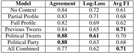
Model Agreement Log-Loss Avg F1
No Context 0.84 0.72 0.61
Partial Profile 0.83 0.71 0.68
Full Profile 0.82 0.69 0.62
Previous Tweets 0.84 0.65 0.71
Political Tweets 0.88 0.61 0.70 Political Party 0.88 0.63 0.68
All Combined 0.77 0.62 0.71
Table 3: Inter-annotator agreement, then perfor-mance of classifier trained on majority vote labels. (Best possible is 1 for agreement and F1, 0 for log-loss.)
intervals.
3.2 Effects of the Contexts
Before evaluating classification results, we con-sider annotator agreement within each context, calculated like Mohammad et al. (2016b) as the average, across tweets, of the percentage of anno-tations that match the majority vote. As shown in Table3, annotators shown No Context achieve an agreement score of 0.84, similar to the 0.8185 reported by Mohammad et al.(2016b). Relative to this baseline, some contexts increase agreement more than others. As one might expect, Previ-ous Political Tweets and Political Party show the strongest signals. Their effects are statistically (p < .01, Mann-Whitney test) and practically sig-nificant, increasing the number of labels having
fullagreement by 15% and 10%, respectively. However, annotators shown different contexts did not necessarily converge to the same labels. Notice the low agreement for the All Combined condition: the majority labels held stronger ma-jorities within any individual context than across all of them. In fact, if we look at the six major-ity vote labels for each tweet, only in 43% of the tweets are these labels in full agreement. At the end of Section5, we return to the question of why agreement was so low across conditions, with the help of parameters estimated by ConStance.
In the classification task, the results in Ta-ble3further suggest that Previous Political Tweets
serves as the strongest single context. There is a good case to be made for choosing this individ-ual context, which is statistically significantly bet-ter than many others. For example, providing an-notators with Previous Political Tweets provides a statistically significant increase in both average F1 scores and log-loss (withp < .01) over both the No Context and Full Profile conditions. Perhaps most noteworthy is that the All Combined classi-fier, created from the naive combination of all an-notations, is no better than the classifiers from the individual conditions.
To summarize, results suggest that providing annotators with appropriate additional context can improve annotation quality, as measured via an-notator agreement and downstream classification performance. However, it was not obvious in ad-vance which context would be most helpful, and performing such an analysis as this requires the time-intensive construction of better “gold stan-dard” labels against which to check the labels al-ready being outsourced to annotators. In addition, the heterogeneity of the labels produced in differ-ent contexts suggests that the contexts provide di-verse signals we might be able to leverage; how-ever, simply combining all the annotations does not result in improvements.
4 ConStance: General Unified Model
The prior section thus suggests that it may be bet-ter to limit a priori decisions and instead to lever-age multiple kinds of context during annotation. LikeRaykar et al. (2010) assumes for annotators, we might expect (and indeed find) that even those contexts that turn out to be worse on some metrics still might be useful for other purposes. Here, we present a model for such an approach.
[image:5.595.73.290.172.257.2]differ-Xi Yi S
ic Rica
! " ℳ
C A
Aicannotators
Ci contexts
N items
Classifier
True label Item feature
[image:6.595.81.284.67.188.2]vector
Figure 1: Graphical model for ConStance.
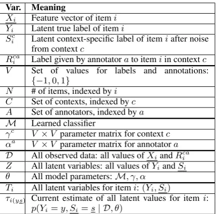
Var. Meaning
Xi Feature vector of itemi
Yi Latent true label of itemi
Sc
i Latent context-specific label of itemiafter noise from contextc
Rca
i Label given by annotatorato itemiin contextc
V Set of values for labels and annotations: {−1,0,1}
N # of items, indexed byi C Set of contexts, indexed byc A Set of annotators, indexed bya
M Learned classifier
γc V ×V parameter matrix for contextc
αa V ×V parameter matrix for annotatora D All observed data: all values ofXiandRcai
Z All latent variables: all values ofYiandSi
θ All model parameters:M, γ, α Ti All latent variables for itemi:(Yi, Si)
τi(ys) Current estimate of all latent values for itemi:
[image:6.595.73.288.226.438.2]p(Yi=y, Si=s| D, θ)
Table 4: Model variables.
ent setup; for example, an item could be a user and ten anchor tweets. However, the current ar-rangement allows for straightforward comparison to prior stance work on Twitter (Mohammad et al.,
2016a).
Note that in general, the features need not be restricted to those annotators could have seen. Rather, they could include anything useful to a classifier. Note also that the feature set provided to ConStance is the same used by the baseline mod-els; only the models themselves differ.
4.1 Overview
The model we develop is shown in Figure1. There are N items to be labeled. Each item can be viewed in up toCdifferent contexts. Finally, there areAtotal annotators labeling the items; each an-notator sees multiple items. Each item can have a different number of annotations, produced by any assignment of annotators and information condi-tions to items. In our dataset, every item is labeled
in 6 conditions (every|Ci|= 6), and within every
context, every item is labeled by at least 3 annota-tors (every|Ac
i| ≥3).
The model’s generative story works as follows. Item i has feature vector Xi and a “true” label
Yi ∈ V. The relationship betweenXi andYi can
be described by some model M, which we will ultimately learn. When the item is viewed with context c, the item’s true labelYi is transformed
by noise into a “context-specific” labelSc
i ∈ V.
In other words, the true label may appear differ-ently when seen through the lens of each context. The variableSc
i represents what an ideal annotator
would say about itemigiven only as much infor-mation as is preserved by contextc.
The “noise” introduced by context c is de-scribed by parameter γc. The parameter γc is a
V ×V matrix of transition probabilities from true labels to context-specific labels. These probabil-ities depend only onYi andγc, not on the item’s
featuresXi.
Importantly, annotators themselves are also im-perfect. When annotator asees item i, she may also distort the label she sees,Sc
i, into the observed
annotationRca
i ∈V. The annotator-specific noise
process is described by parameter αa, another
V ×V transition matrix.
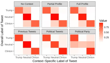
For a better understanding of the role of γc
(and by anology, αa), consider the depictions in
Figure 2. The matrix on the top left refers to the No Context condition. Its top row describes what an annotator with perfect judgment would think about a user whose true label is Trump [sup-porter], with no context. The top left cell, with a value around 0.65, is the probability the annotator would think Trump; the lighter middle cell, with a value around 0.35, is the probability she would think Neutral/Don’t know; and the probability she would think Clinton is almost 0.
4.2 Learning
Like Raykar et al. (2010), we perform infer-ence using Expectation Maximization (EM). A full derivation is provided in the Supplementary Material; here, we sketch the main steps.
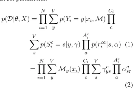
The model’s incomplete data likelihood func-tion, Eq. (1), describes the joint probability, across all items, ofYi, all values ofSic, and all values of
Rca
i assumingXi is known and fixed. Uppercase
model parameters.
p(D|θ, X) =YN
i=1
V
X
y
p(Yi =y|xi,M) Ci Y
c V
X
s
p(Sic=s|y, γ)
Ac i Y
a
p(rica|s, α) (1)
=YN
i=1
V
X
y
My(xi) Ci Y
c V
X
s
γcys
Ac i Y
a
αasr
(2) The EM derivation is difficult because both Yi
andSiare unobserved. Our solution is to treat the
latent variables as a block, describing their joint configuration with a single termTi = (Yi, Si). In
our data, since|Ci|= 6,Ti can take on7|V|
pos-sible values, a number small enough to enumerate over when we need to marginalize outTi.
We define membership indicator variables Ti(ys) ∈ {0,1} such that Ti(ys) = 1 if Ti has
the specific values (y, s). During learning, we use analogous variablesτi(ys)∈[0,1]to represent the posterior probabilities of each configuration: τi(ys) =p(Ti(ys)= 1 | D, θ). The expected value of the complete data log-likelihood is:
EZ[`(D, Z|θ, X)] = N
X
i=1
V
X
y
V
X
s1 i
. . .XV
sCii
τi(ys)(logp(Ti(ys)|xi,M, γ) + Ci X
c Ac
i X
a
logαa sr)
(3) For the E step, we update the membership esti-matesτi(ys) using the current parametersθ. With Bayes’ rule, each item’s new value of τi(ys) is shown to be the full joint likelihood of itemi(see Eq. (2)) when settingYi =yandSi =s, divided
by the sum, over all possible settings ofYi andSi,
of that same joint likelihood.
For the M step, we update the model parame-ters using the current membership estimates. To update the classifier M, following the guidance ofRaykar et al. (2010), we retrain the classifier using the current estimates of Yi as weights for
items. The estimates of Yi can be obtained from
τiys by marginalizing outSi, thusEZ[Yi = y] =
PV
s1 i . . .
PV
sCii τiys. We then use sampling to
con-struct a discrete set of labels for model training based on these weights.
Model Log-Loss Avg F1
Best baselines 0.61 0.71
ConStance 0.57 0.77
Ablations
[image:7.595.76.292.73.216.2]1. Only Political Tweets 0.59 0.73 2. Context Labels Masked 0.57 0.75 3. Annotator Labels Masked 0.65 0.75
Table 5: Classification performance of ConStance and model ablations. Boldface highlights best scores. Significance tests use the the p < .05 level for log-loss. Compared to the best baselines, all scores that appear better are statistically signif-icant. Italics indicate the scores that are signifi-cantly worse than ConStance.
To updateγ andα, we maximize them with re-spect to Eq. (3). Forγ, the entryγc
ys(i.e., rowy,
columnsof matrix γc) denotesp(Sc
i = s| Yi =
y). Each matrix entry can be updated individually by taking the partial derivative of Eq. (3) and us-ing, as a Lagrange multiplier term, the constraint that the row must sum to 1. The updated value for γc
ysturns out to be a fraction in which the
numera-tor is the weighted (byτ) number of items having Yi = y andSic = s, and the denominator is the
weighted number of items havingYi=y(and any
value for Sc
i). For α, a similar derivation yields
the following update toαa
sr: the weighted number
of labels by annotator a, in any context, having Sc
i = sand Rcai = r, divided by the weighted
number of labels by annotator a, in any context, havingSc
i =s.
5 Model Results and Discussion
The top portion of Table 5 displays ConStance’s performance compared to the best results from Section3. Using the same experimental setup as Section 3—the model type and features, M and Xrespectively, are the same as in the baselines— ConStance improves over the best baseline mod-els for each metric. This improvement is statisti-cally significant for both metrics (at thep < .05 level for log-loss). Further, the model converges rapidly, within 5-7 iterations of the EM algorithm and 3-5 minutes on a single machine.2
In addition to comparing to the baselines pro-vided in Section3, we investigate which informa-tion the model is leveraging to be successful. We do so by exploring three ablations of the model. Variation #1 (“Only Political Tweets” in Table5)
2As above, a development set is used for coarse
uses the full model, but only gives it the annota-tions from the Political Tweets condition. This tests whether simply modeling differences in an-notators’ error rates, as Raykar et al. (2010) do, with a single (“best”) context is helpful. We find that it is: the performance of this variation is sig-nificantly better on both metrics than the Political Tweets baseline from Table3.
In the second and third variations, we check whether the effectiveness of ConStance stems from modeling differences between annotators rather than differences in contexts, or vice versa. Variation #2 (“Context Labels Masked”), like #1, models only annotator effects; however, it instead uses the entire set of annotations, treating them as if from a single context (i.e., “masking” context in-formation from the model). Variation #3 (“Anno-tator Labels Masked”) is the complement of Vari-ation #2: it models differences in contexts, and it uses the entire set of annotations, treating them as if from a single annotator.
The results of the model ablation experiments are three-fold. First, we see that each piece of the model on its own is effective in moving beyond baseline approaches that use only one context or naively combine labels across contexts and anno-tators (the “All Combined” baseline). All model variations achieve significantly higher Avg. F1 than the baselines, and Variations #1 and #2 im-prove on log-loss. Second, we see that model-ing annotators alone is clearly better than not: not only does Variation #1 outperform the Political Tweets baseline (significantly), but also Variation #2 outperforms the All Combined baseline (signif-icantly) and ConStance outperforms Variation #3 (with significance in one measure). Finally, the best results come from using the full model. Even if the differences between ConStance and the vari-ations are not all statistically significant, model-ing both annotators and contexts appears to be the most complete and effective approach.
In addition to model performance, we can also examine what ConStance has learned about the quality of labels from each context. Recall that the model produces a parameter matrix for each con-text,γc, which describes how a context distorts the
“true” labels the model assumes. Eachγcis a
tran-sition matrix, so a context that perfectly preserves true labels would show up as the identity matrix; off-diagonal entries show error patterns.
Figure 2 visualizes parameter estimates for γ.
Previous Tweets Political Tweets Political Party No Context Partial Profile Full Profile
Trump Neutral Clinton Trump Neutral Clinton Trump Neutral Clinton Clinton
Neutral Trump
Clinton Neutral Trump
Context−Specific Label of Tweet
Ov
er
all Label of T
w
eet
0.25 0.50 0.75
[image:8.595.309.522.63.185.2]Value
Figure 2: Parameter matricesγclearned by
Con-Stance for each context. Darker shading indicates higher values.
We see that in the No Context, Partial Profile and Full Profile conditions, annotators often selected the “Neutral” option (x-axis) when the model in-ferred the true label was “Clinton” or “Trump” (y -axis). This finding is in line with intuitions; an-notators who saw these conditions simply lacked enough information to determine any label.
On the other extreme, in the Political Party con-text, annotators selected “Trump” or “Clinton” too often when the model settled on the “Neutral” op-tion. That is, even when a user’s stance was not clear to annotators in other conditions, annotators who saw political party still inferred stance from the text. Here, one could argue annotators were shown “too much” or “too strong” a context—they saw stance even where the content produced by the user did not suggest one. Indeed, further manual inspection of 90 tweets on which annotations dis-agreed across contexts implies that annotators who saw political affiliation were often wrong because they focused too little on text content relative to the provided political affiliations.
In presenting these findings, a key point to high-light is that unlike the results of Section3, Figure2
was produced without access to any full informa-tion labels, which depend on a significant level of manual effort beyond annotations gathered on AMT.
6 Related Work
Recent work has shown that cognitive biases such as stereotypes (Carpenter et al.,2016) and anchor-ing (Berzak et al., 2016) can negatively impact text annotation and resulting models, even for ob-jective tasks like POS tagging (Blodgett et al.,
evalu-ating how their decisions will affect annotations, on tasks from gender identification to political leanings (Chen et al., 2015;Nguyen et al.,2014;
Burger et al.,2011;Cohen and Ruths,2013). Our work suggests an interesting avenue of develop-ment towards reducing annotation bias by explic-itly modeling it and reducing the need for a priori decisions on which context is best for which par-ticular task.
In doing so, we draw on a large body of work around improving annotation quality for NLP data. Our work aligns with efforts to improve task design (e.g.Schneider et al.,2013;Morstatter and Liu, 2016;Schneider, 2015), and to develop better models of annotation. With respect to the former and specific to Twitter,Frankenstein et al.
(2016) show that for the task of labeling the senti-ment of reply tweets, annotations vary depending on whether or not the original tweet (being replied to) is also shown. With respect to the latter, sev-eral recent models beyond Raykar et al. (2010) have been proposed (Guan et al.,2017;Tian and Zhu, 2012; Wauthier and Jordan, 2011; Passon-neau and Carpenter,2014). However, our work is most similar to efforts outside the domain of NLP, whereDai et al.(2013) have developed a method of switching between task workflows based on an-notation quality for particular items, and Nguyen et al. (2016) have developed a Bayesian model similar to ours to study annotation quality for other kinds of slightly subjective tasks.
In a closely related vein, recent work has also considered how text annotations may vary in im-portant ways based on the characteristics of anno-tators (rather than how the task is posed, as we study here) (Sen et al.,2015). An interesting av-enue of future work is to understand the intersec-tion between the design of NLP annotaintersec-tion tasks and the characteristics of the annotating popula-tion.
7 Conclusion and Future Work
Annotated data serves as a foundational layer for many NLP tasks. While some annotation tasks only require information from short texts, in many others, we can elicit higher-quality labels by pro-viding annotators with additional contextual infor-mation. However, asking annotators to consider too much information would make their task slow and burdensome.
In this paper we demonstrate how exposing
an-notators to short contextual information leads to better labels and better classification results. How-ever, different contexts lead to results of different quality, and it is not obvious a priori which con-text is best, nor—even given ground truth—how to combine labels produced across contexts to ex-ploit the information present in each. We then pro-pose ConStance, a generalizable model that learns the effects of both individual contexts and individ-ual annotators on the labeling process. The model infers (probability estimates for) ground truth la-bels, plus learns a classifier that can be applied to new instances. We show that this classifier signif-icantly improves classification of political stance compared to the standard practice of training mod-els on majority vote labmod-els.
The focus of this work is on improving both the annotation process for nuanced, context-dependent tasks and the use of the resulting labels. While ConStance’s label estimation can be used in conjunction with any classification method, this paper does not address the optimization of the classifier itself. Thus, while we consider an as-sortment of contexts and use a rich feature rep-resentation, using additional contexts or different features may lead to better performance on stance detection. Finally, the model is versatile enough we could consider treating different tweets as dif-ferent “contexts” for the same user, augmenting the extensively annotated tweets with other types of data, and, naturally, applying the same frame-work to other annotation tasks.
References
Pablo Barber´a. 2016. Less is more? How demo-graphic sample weights can improve public opinion estimates based on Twitter data. Working Paper.
Yevgeni Berzak, Yan Huang, Andrei Barbu, Anna Ko-rhonen, and Boris Katz. 2016. Anchoring and Agreement in Syntactic Annotations.arXiv preprint arXiv:1605.04481.
Su Lin Blodgett, Lisa Green, and Brendan O’Connor. 2016. Demographic dialectal variation in social me-dia: A case study of African-American English.
EMNLP’16.
Jordan Carpenter, Daniel Preot¸iuc-Pietro, Lucie Flekova, Salvatore Giorgi, Courtney Hagan, Mar-garet Kern, Anneke E. K. Buffone, Lyle Ungar, and Martin E. P. Seligman. 2016. Real Men Don’t Say “Cute”: Using Automatic Language Analysis to Iso-late Inaccurate Aspects of Stereotypes. Social Psy-chological and Personality Science.
Xin Chen, Yu Wang, Eugene Agichtein, and Fusheng Wang. 2015. A Comparative Study of Demographic Attribute Inference in Twitter. ICWSM, 15:590–593.
Raviv Cohen and Derek Ruths. 2013. Classifying po-litical orientation on Twitter: It’s not easy! In
ICWSM.
Peng Dai, Christopher H. Lin, Mausam, and Daniel S. Weld. 2013. POMDP-based control of workflows for crowdsourcing. Artificial Intelligence, 202:52– 85.
Paul DiMaggio. 2015. Adapting computational text analysis to social science (and vice versa). Big Data & Society, 2(2).
Javid Ebrahimi, Dejing Dou, and Daniel Lowd. 2016. A Joint Sentiment-Target-Stance Model for Stance Classification in Tweets. COLING’16.
Will Frankenstein, Kenneth Joseph, and K. M. Carley. 2016. Contextualized Sentiment Analysis. In So-cial Computing, Behavioral-Cultural Modeling and Prediction, Washington, DC, USA.
Melody Y. Guan, Varun Gulshan, Andrew M. Dai, and Geoffrey E. Hinton. 2017. Who Said What: Mod-eling Individual Labelers Improves Classification.
arXiv:1703.08774 [cs].
William Hobbs, Lisa Friedland, Kenneth Joseph, Oren Tsur, Stefan Wojcik, and David Lazer. 2017. “Vot-ers of the Year”: 19 Vot“Vot-ers Who Were Unintentional Election Poll Sensors on Twitter. InICWSM.
C. J. Hutto and Eric Gilbert. 2014. Vader: A parsimo-nious rule-based model for sentiment analysis of so-cial media text. InEighth International AAAI Con-ference on Weblogs and Social Media.
Kenneth Joseph, Wei Wei, and Kathleen M. Carley. 2017. Girls rule, boys drool: Extracting seman-tic and affective stereotypes from Twitter. In 2017 ACM Conference on Computer Supported Coopera-tive Work.(CSCW).
Saif M. Mohammad, Svetlana Kiritchenko, Parinaz Sobhani, Xiaodan Zhu, and Colin Cherry. 2016a. Semeval-2016 task 6: Detecting stance in tweets. In
Proceedings of the International Workshop on Se-mantic Evaluation, SemEval, volume 16.
Saif M. Mohammad, Parinaz Sobhani, and Svetlana Kiritchenko. 2016b. Stance and sentiment in tweets.
arXiv preprint arXiv:1605.01655.
Fred Morstatter and Huan Liu. 2016. Replacing me-chanical turkers? challenges in the evaluation of models with semantic properties. Journal of Data and Information Quality (JDIQ), 7(4):15.
An Thanh Nguyen, Matthew Halpern, Byron C. Wal-lace, and Matthew Lease. 2016. Probabilistic mod-eling for crowdsourcing partially-subjective ratings. InProceedings of The Conference on Human Com-putation and Crowdsourcing (HCOMP), pages 149– 158.
Dong Nguyen, Rilana Gravel, Dolf Trieschnigg, and Theo Meder. 2013. “How Old Do You Think I Am?”: A Study of Language and Age in Twitter. In
Seventh International AAAI Conference on Weblogs and Social Media.
Dong-Phuong Nguyen, R. B. Trieschnigg, A. Seza Do˘gru¨oz, Rilana Gravel, Mari¨et Theune, Theo Meder, and F. M. G. de Jong. 2014. Why gender and age prediction from tweets is hard: Lessons from a crowdsourcing experiment. InProceedings of COL-ING 2014.
Rebecca J. Passonneau and Bob Carpenter. 2014. The benefits of a model of annotation. Transactions of the Association for Computational Linguistics, 2:311–326.
Vikas C. Raykar, Shipeng Yu, Linda H. Zhao, Ger-ardo Hermosillo Valadez, Charles Florin, Luca Bogoni, and Linda Moy. 2010. Learning from crowds. Journal of Machine Learning Research, 11(Apr):1297–1322.
Nathan Schneider. 2015. What I’ve learned about an-notating informal text (and why you shouldn’t take my word for it). In The 9th Linguistic Annotation Workshop Held in Conjuncion with NAACL 2015, page 152.
Nathan Schneider, Brendan O’Connor, Naomi Saphra, David Bamman, Manaal Faruqui, Noah A. Smith, Chris Dyer, and Jason Baldridge. 2013. A frame-work for (under) specifying dependency syntax without overloading annotators. arXiv preprint arXiv:1306.2091.
Shilad Sen, Isaac L. Johnson, Rebecca Harper, Huy Mai, Samuel Horlbeck Olsen, Benjamin Math-ers, Laura Souza Vonessen, Matthew Wright, and Brent J. Hecht. 2015. Towards Domain-Specific Se-mantic Relatedness: A Case Study from Geography. InIJCAI, pages 2362–2370.
Yuandong Tian and Jun Zhu. 2012. Learning from crowds in the presence of schools of thought. In
Proceedings of the 18th ACM SIGKDD Interna-tional Conference on Knowledge Discovery and Data Mining, pages 226–234. ACM.