Learning to Predict Denotational Probabilities For Modeling Entailment

(1)

Learning to Predict Denotational Probabilities For Modeling Entailment

Alice Lai and Julia Hockenmaier Department of Computer Science University of Illinois at Urbana-Champaign {aylai2, juliahmr}@illinois.edu

Abstract

We propose a framework that captures the denotational probabilities of words and phrases by embedding them in a vector space, and present a method to induce such an embedding from a dataset of denota-tional probabilities. We show that our model successfully predicts denotational probabilities for unseen phrases, and that its predictions are useful for textual entail-ment datasets such as SICK and SNLI.

1 Introduction

In order to bridge the gap between vector-based distributional approaches to lexical semantics that are intended to capture which words occur in sim-ilar contexts, and logic-based approaches to com-positional semantics that are intended to capture the truth conditions under which statements hold, Young et al. (2014) introduced the concept of “denotational similarity.” Denotational similarity is intended to measure the similarity of simple, declarative statements in terms of the similarity of their truth conditions.

From classical truth-conditional semantics, Young et al. borrowed the notion of the

deno-tation of a declarative sentence s, JsK, as the set

of possible worlds in which the sentence is true. Young et al. apply this concept to the domain of

image descriptions by defining thevisual

denota-tionof a sentencesas the set of images thats

de-scribes. The denotational probability ofs,PJK(s),

is the number of images in the visual denotation

ofsover the size of the corpus. Two sentences are

denotationally similar if the sets of images (possi-ble worlds) they describe have a large overlap. For example, “A woman is jogging on a beach” and “A woman is running on a sandy shore” can of-ten be used to describe the same scenario, so they

will have a large image overlap that corresponds to high denotational similarity.

Given the above definitions, Young et al. es-timate the denotational probabilities of phrases

from FLICKR30K, a corpus of 30,000 images,

each paired with five descriptive captions. Young et al. (2014) and Lai and Hockenmaier (2014) showed that these similarities are complementary to standard distributional similarities, and poten-tially more useful for semantic tasks that involve entailment. However, the systems presented in these papers were restricted to looking up the de-notational similarities of frequent phrases in the training data. In this paper, we go beyond this

prior work and define a model that can predict

the denotational probabilities of novel phrases and sentences. Our experimental results indicate that these predicted denotational probabilities are use-ful for several textual entailment datasets.

2 Textual entailment in SICK and SNLI

The goal of textual entailment is to predict whether a hypothesis sentence is true, false, or neither based on the premise text (Dagan et al., 2013). Due in part to the Recognizing Textual Entailment (RTE) challenges (Dagan et al., 2006), the task of textual entailment recognition has received a lot of attention in recent years. Although full entail-ment recognition systems typically require a com-plete NLP pipeline, including coreference resolu-tion, etc., this paper considers a simplified variant of this task in which the premise and hypothesis are each a single sentence. This simplified task allows us to ignore the complexities that arise in longer texts, and instead focus on the purely se-mantic problem of how to represent the meaning of sentences. This version of the textual entail-ment task has been popularized by two datasets, the Sentences Involving Compositional

(2)

edge (SICK) dataset (Marelli et al., 2014) and the Stanford Natural Language Inference (SNLI) cor-pus (Bowman et al., 2015), both of which involve a 3-way classification for textual entailment.

SICK was created for SemEval 2014 based on image caption data and video descriptions. The premises and hypotheses are automatically gen-erated from the original captions and so contain some unintentional systematic patterns. Most ap-proaches to SICK involve hand-engineered fea-tures (Lai and Hockenmaier, 2014) or large col-lections of entailment rules (Beltagy et al., 2015). SNLI is the largest textual entailment dataset by several orders of magnitude. It was created with the goal of training neural network models for tex-tual entailment. The premises in SNLI are

cap-tions from the FLICKR30K corpus (Young et al.,

2014). The hypotheses (entailed, contradictory, or neutral in relation to the premise) were solicited from workers on Mechanical Turk. Bowman et al. (2015) initially illustrated the effectiveness of LSTMs (Hochreiter and Schmidhuber, 1997) on SNLI, and recent approaches have focused on im-provements in neural network architectures. These include sentence embedding models (Liu et al., 2016; Munkhdalai and Yu, 2017a), neural atten-tion models (Rockt¨aschel et al., 2016; Parikh et al., 2016), and neural tree-based models (Munkhdalai and Yu, 2017b; Chen et al., 2016). In contrast, in this paper we focus on using a different input representation, and demonstrate its effectiveness when added to a standard neural network model for textual entailment. We demonstrate that the re-sults of the LSTM model of Bowman et al. (2015) can be improved by adding a single feature based on our predicted denotational probabilities. We expect to see similar improvements when our pre-dicted probabilities are added to more complex neural network entailment models, but we leave those experiments for future work.

3 Vector space representations

Several related works have explored different ap-proaches to learning vector space representations that express entailment more directly. Kruszewski et al. (2015) learn a mapping from an existing distributional vector representation to a structured Boolean vector representation that expresses en-tailment as feature inclusion. They evaluate the resulting representation on lexical entailment tasks and on sentence entailment in SICK, but they

re-strict SICK to a binary task and their sentence vectors result from simple composition functions (e.g. addition) over their word representations. Henderson and Popa (2016) learn a mapping from an existing distributional vector representa-tion to an entailment-based vector representarepresenta-tion that expresses whether information is known or unknown. However, they only evaluate on lexical semantic tasks such as hyponymy detection.

Other approaches explore the idea that it may be more appropriate to represent a word as a re-gion in space instead of a single point. Erk (2009) presents a word vector representation in which the hyponyms of a word are mapped to vectors that exist within the boundaries of that word vector’s region. Vilnis and McCallum (2015) use Gaussian functions to map a word to a density over a latent space. Both papers evaluate their models only on lexical relationships.

4 Denotational similarities

In contrast to traditional distributional similarities, Young et al. (2014) introduced the concept of “de-notational similarities” to capture which expres-sions can be used to describe similar situations.

Young et al. first define thevisual denotation of

a sentence (or phrase) s, JsK, as the (sub)set of

images that s can describe. They estimate the

denotation of a phrase and the resulting

similar-ities from FLICKR30K, a corpus of 30,000

im-ages, each paired with five descriptive captions. In order to compute visual denotations from the corpus, they define a set of normalization and re-duction rules (e.g. lemmatization, dropping modi-fiers, replacing nouns with their hypernyms, drop-ping PPs, extracting NPs) that augment the

origi-nal FLICKR30K captions with a large number of

shorter, more generic phrases that are each

associ-ated with a subset of the FLICKR30K images.

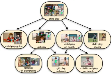
The result is a large subsumption hierarchy over phrases, which Young et al. call a denotation graph (see Figure 1). The structure of the deno-tation graph is similar to the idea of an entailment graph (Berant et al., 2012). Each node in the

de-notation graph corresponds to a phrases,

associ-ated with its denotation JsK, i.e. the set of

im-ages that correspond to the original captions from which this phrase could be derived. For example,

the denotation of a phrase“woman jog on beach”

(3)

deno-child play   soccer child play guitar

child in red play   on beach girl play  

on beach child play   on beach girl play

girl play   on playground

[image:3.595.88.281.64.194.2]

child play

Figure 1: The denotation graph is a subsumption hierarchy over phrases associated with images.

tation of a node (e.g. “woman jog on beach”) is

always a subset of the denotations of any of its

an-cestors (e.g. “woman jog”,“person jog”,“jog on

beach”, or“beach”).

The denotational probability of a phrase s,

PJK(s), is a Bernoulli random variable that

corre-sponds to the probability that a randomly drawn

image can be described bys. Given a denotation

graph overN images, PJK(s) = |JsK|N . The joint

denotational probability of two phrases x and y,

P_JK(x, y) = |JxK∩JyK|_N , indicates how likely it is

that a situation can be described by both x and

y. Young et al. propose to use pointwise mu-tual information scores (akin to traditional distri-butional similarities) and conditional probabilities P_JK(x|y) = |JxK∩JyK|_|JyK| as so-called denotational sim-ilarities. In this paper, we will work with de-notational conditional probabilities, as they are intended to capture entailment-like relations that hold due to commonsense knowledge, hyponymy,

etc. (what is the probability that x is true, given

thatycan be said about this situation?). In an ideal

scenario, if the premise p entails the hypothesis

h, then the conditional probabilityP(h|p)is 1 (or

close to 1). Conversely, ifhcontradictsp, then the

conditional probability P(h|p) is close to 0. We

therefore stipulate that learning to predict the

con-ditional probability of one phrasehgiven another

phrasepwould be helpful in predicting textual

en-tailment. We also note that by the definition of the

denotation graph, if x is an ancestor of y in the

graph, thenyentailsxandPJK(x|y) = 1.

Young et al. (2014) and Lai and Hockenmaier (2014) show that denotational probabilities can be at least as useful as traditional distributional sim-ilarities for tasks that require semantic inference such as entailment or textual similarity recogni-tion. However, their systems can only use

deno-o x1

x2

y

x

P(X,Y) P(X)

o x1

x2

y z x

P(X,Y)

P(Y) P(X)

Figure 2: An embedding space that expresses the

individual probability of eventsX andY and the

joint probabilityP(X, Y).

tational probabilities between phrases that already exist in the denotation graph (i.e. phrases that

can be derived from the original FLICKR30K

cap-tions).

Here, we present a model that learns to

pre-dict denotational probabilitiesPJK(x)andPJK(x|y)

even for phrases it has not seen during training. Our model is inspired by Vendrov et al. (2016),

who observed that a partial ordering over the

vector representations of phrases can be used to express an entailment relationship. They induce a so-called order embedding for words and phrases

such that the vectorxcorresponding to phrase x

is smaller than the vector y, i.e. x y, for

phrases y that are entailed by x, where

cor-responds to the reversed product order on RN

+ (

x y ⇔ xi ≥ yi∀i). They use their model

to predict entailment labels between pairs of sen-tences, but it is only capable of making a binary entailment decision.

5 An order embedding for probabilities We generalize this idea to learn an embedding space that expresses not only the binary relation

that phrasexis entailed by phrasey, but also the

probability that phrase x is true given phrase y.

Specifically, we learn a mapping from a phrasex

to anN-dimensional vectorx∈RN

+ such that the

vectorx = (x1, ..., xN) defines the denotational

probability ofx asP_JK(x) = exp(−P_ixi). The

origin (the zero vector) therefore has probability

exp(0) = 1. Any other vector x that does not

lie on the origin (i.e. ∃ixi > 0) has probability

less than 1, and a vectorxthat is farther from the

origin than a vector y represents a phrase x that

[image:3.595.319.513.66.144.2]

(4)

pro-portional to the entire region of the positive or-thant, while other points in the space correspond to smaller regions and thus probabilities less than 1.

The joint probability PJK(x, y) in this

embed-ding space should be proportional to the size of

the intersection of the regions ofxandy.

There-fore, we define the joint probability of two phrases

x and y to correspond to the vector z that is

the element-wise maximum of x and y: zi =

max(xi, yi). This allows us to compute the

con-ditional probabilityP_JK(x|y)as follows:

P_JK(x|y) = P_PJK(x, y) JK(y)

= exp(−

P

izi) exp(−P_iyi)

= exp(X

i

yi−

X

i

zi)

Shortcomings We note that this embedding

does not allow us to represent the negation ofxas

a vector. We also cannot represent two phrases that have completely disjoint denotations: in Figure 2,

theP(X)andP(Y)regions will always intersect

and therefore theP(X, Y)region will always have

an area greater than 0. In fact, in our embedding space, the joint probability represented by the

vec-tor z will always be greater than or equal to the

product of the probabilities represented by the

vec-torsxandy. For any pair x = (x1, ..., xN) and

y= (y1, ..., yN),PJK(X, Y)≥PJK(X)PJK(Y):

P_JK(X, Y) = exp −X

i

max(xi, yi)

≥exp −X

i

xi−

X

i

yi

=P_JK(X)P_JK(Y)

(Equality holds when x and y are

orthogo-nal, and thusP_ixi+Piyi = Pimax(xi, yi)).

Therefore, the best we can do for disjoint phrases is learn an embedding that assumes the phrases are independent. In other words, we can map the dis-joint phrases to two vectors whose computed dis-joint probability is the product of the individual phrase probabilities.

Although our model cannot represent two events with completely disjoint denotations, we will see below that it is able to learn that some phrase pairs have very low denotational condi-tional probabilities. We note also that our model

… …

w0 wi wi+1 wN

Glove

embeddings

LSTM RNN 512D FF

p(x)

LSTM is run once per phrasex, y

p(y)

p(x|y)

Predictions trained with Cross Entropy

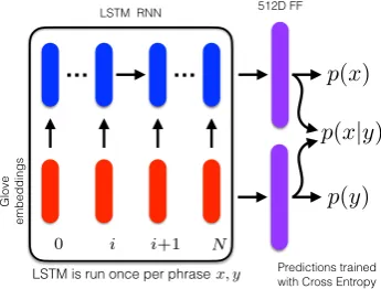
Figure 3: Our probability model architecture. Each phrase is a sequence of word embeddings that is passed through an LSTM to produce a 512d vector representation for the premise and the hy-pothesis. Both vectors are used to compute the predicted conditional probability and calculate the loss.

cannot expressP(X) = 0exactly, but can get

ar-bitrarily close in order to represent the probability of a phrase that is extremely unlikely.

6 Our model forPJK(x)andPJK(x, y)

We train a neural network model to predictPJK(x),

P_JK(y), and P_JK(x|y) for phrases x and y. This

model consists of an LSTM that outputs a 512d vector which is passed through an additional 512d layer. We use 300d GloVe vectors (Pennington et al., 2014) trained on 840B tokens as the word embedding input to the LSTM. We use the same

model to represent both x and y regardless of

which phrase is the premise or the hypothesis. Thus, we pass the sequence of word embeddings

for phrase xthrough the model to get x, and we

do the same for phraseyto gety. As previously

described, we sum the elements ofxandyto get

the predicted denotational probabilitiesP_JK(x)and

P_JK(y). From x and y, we find the joint vector

z, which we use to compute the predicted

denota-tional condidenota-tional probability P_JK(x|y) according

to the equation in Section 5. Figure 3 illustrates the structure of our model.

Our training data consists of ordered phrase

pairs hx, yi. We train our model to predict the

denotational probabilities of each phrase (PJK(x)

andP_JK(y)) as well as the conditional probability

PJK(x|y). Typically the pairhy, xiwill also appear

in the training data.

Our per-example loss is the sum of the cross

[image:4.595.330.503.63.194.2]

(5)

L= −

PJK(x) logQ(x) + (1−PJK(x)) log 1−Q(x)

−_P

JK(y) logQ(y) + (1−PJK(y)) log 1−Q(y)

−_P

JK(x|y) logQ(x|y) + (1−PJK(x|y)) log 1−Q(x|y)

We use the Adam optimizer with a learning rate of 0.001, and a dropout rate of 0.5. These param-eters were tuned on the development data.

Numerical issues In Section 5, we described the

probability vectorsx as being in the positive

or-thant. However, in our implementation, we use unnormalized log probabilities. This puts all of our vectors in the negative orthant instead, but it prevents the gradients from becoming too small during training. To ensure that the vectors are

in RN

−, we clip the values of the elements of x

so that xi ≤ 0. To compute logPJK(x), we

sum the elements of x and clip the sum to the

range(log(10−10₎_,₋₀_.₀₀₀₁₎_{in order to avoid}

er-rors caused by passing log(0) values to the loss

function. The conditional log probability is simply

logP_JK(x|y) = logP_JK(x, y)−logP_JK(y), where

logPJK(x, y)is now the element-wise minimum:

logP_JK(x, y) =X i

min(xi, yi)

This element-wise minimum is a standard pool-ing operation (we take the minimum instead of the

more common max pooling). Note that ifxi > yi,

neither elementxi noryi is updated with respect

to the P_JK(x|y) loss. Both xi andyi will always

be updated with respect to thePJK(x) andPJK(y)

components of the loss. 6.1 Training regime

To train our model, we use phrase pairshx, yifrom

the denotation graph generated on the training split

of the FLICKR30K corpus (Young et al., 2014).

We consider all 271,062 phrases that occur with at least 10 images in the training split of the graph, to ensure that the phrases are frequent enough that their computed denotational probabilities are

reli-able. Since the FLICKR30K captions are

lemma-tized in order to construct the denotation graph, all the phrases in the dataset described in this section are lemmatized as well.

We include all phrase pairs where the two phrases have at least one image in common. These

constitute 45 million phrase pairs hx, yi with

PJK(x|y) > 0. To train our model to predict

P_JK(x|y) = 0, we include phrase pairshx, yithat

have no images in common ifN×P_JK(x)P_JK(y)≥

N−1 _(N _{is the total number of images),}

mean-ing thatx andy occur frequently enough that we

would expect them to co-occur at least once in the

data. This yields 2 million pairs wherePJK(x|y) =

0. For additional examples of P_JK(x|y) = 1,

we include phrase pairs that have an ancestor-descendant relationship in the denotation graph. We include all ancestor-descendant pairs where each phrase occurs with at least 2 images, for an additional 3 million phrase pairs.

For evaluation purposes, we first assign 5% of the phrases to the development pool and 5% to the test pool. The actual test data then consists of all phrase pairs where at least one of the two phrases comes from the test pool. The resulting test data contains 10.6% unseen phrases by type and 51.2% unseen phrases by token. All phrase pairs in the test data contain at least one phrase that was un-seen in the training or development data. The de-velopment data was created the same way.

This dataset is available to download at http://nlp.cs.illinois.edu/ HockenmaierGroup/data.html.

We train our model on the training data (42 million phrase pairs) with batch size 512 for 10 epochs, and use the mean KL divergence on the conditional probabilities in the development data

to select the best model. Since P_JK(x|y) is a

Bernoulli distribution, we compute the KL

diver-gence for each phrase pairhx, yias

DKL(P||Q) =PJK(x|y) logP_QJK₍(_xx_||_yy₎)

+ 1−P_JK(x|y)log1−PJK(x|y) 1−Q(x|y)

where Q(x|y) is the conditional probability

pre-dicted by our model.

7 Predicting denotational probabilities 7.1 Prediction on new phrase pairs

We evaluate our model using 1) the KL

di-vergences DKL(P||Q) of the gold individual

and conditional probabilitiesP_JK(x)andP_JK(x|y)

against the corresponding predicted probabilities

Q, and 2) the Pearson correlation r, which

ex-presses the correlation between two variables (the per-item gold and predicted probabilities) as a

(6)

P(x) P(x|y)

KL r KL r

Training data 0.0003 0.998 0.017 0.974

Full test data 0.001 0.979 0.031 0.949

Unseen pairs 0.002 0.837 0.048 0.920

[image:6.595.76.286.64.154.2]

Unseen words 0.016 0.906 0.127 0.696

Table 1: Our model predicts the probability of un-seen phrase pairs with high correlation to the gold probabilities.

0 0.25 0.5 0.75 1

0 0.1 0.2 0.3 0.4 0.5 0.6 0.7 0.8 0.9

(a) Predicted probability whenPJK(x|y) = 0

0 0.25 0.5 0.75 1

0 0.1 0.2 0.3 0.4 0.5 0.6 0.7 0.8 0.9

(b) Predicted probability whenPJK(x|y) = 0

Figure 4: Predicted probabilities on denotational

phrase test data when PJK(x|y) = 0 is 0 or 1.

Black is the full test data and gray is the subset of pairs where both phrases are unseen. Frequency is represented as a percentage of the size of the data.

1 (total positive correlation). As described above, we compute the KL divergence on a per-item ba-sis, and report the mean over all items in the test set.

Table 1 shows the performance of our trained model on unseen test data. The full test data consists of 4.6 million phrase pairs, all of which contain at least one phrase that was not observed in either the training or development data. Our model does reasonably well at predicting these conditional probabilities, reaching a correlation of

r= 0.949withPJK(x|y)on the complete test data.

On the subset of 123,000 test phrase pairs where both phrases are previously unseen, the model’s

predictions are almost as good atr= 0.920.

On the subset of 3,100 test phrase pairs where at

0 0.1 0.2 0.3

[image:6.595.317.516.65.207.2]

1 2 3 4 5 6 7 8 9 10 11

Figure 5: Distribution of phrase lengths as a frac-tion of the data size on the denotafrac-tion graph phrase training data.

least one word was unseen in training, the model’s

predictions are worse, predicting PJK(x|y) with a

correlation of r = 0.696. On the remaining test

pairs, the model predictsP_JK(x|y)with a

correla-tion ofr = 0.949.

We also analyze our model’s accuracy on phrase

pairs where the goldPJK(x|y)is either 0 or 1. The

latter case reflects an important property of the

de-notation graph, sinceP_JK(x|y) = 1whenx is an

ancestor of y. More generally, we can interpret

PJK(h|p) = 1 as a confident prediction of

entail-ment, andP_JK(h|p) = 0 as a confident prediction

of contradiction. Figure 4 shows the distribution of predicted conditional probabilities for phrase

pairs where gold P_JK(h|p) = 0 (top) and gold

P_JK(h|p) = 1(bottom). Our model’s predictions on unseen phrase pairs (gray bars) are nearly as ac-curate as its predictions on the full test data (black bars).

7.2 Prediction on longer sentences

[image:6.595.101.260.215.455.2]

(7)

explicit negation. We augment the SNLI data with approximate gold denotational probabilities by

as-signing a probabilityPJK(S) =s/N to a sentence

Sthat occursstimes in theN training sentences.

We assign approximate gold conditional

probabil-ities for each sentence pairhp, hiaccording to the

entailment label: ifpentailsh, thenP(h|p) = 0.9.

Ifp contradictsh, thenP(h|p) = 0.001.

Other-wise,P(h|p) = 0.5.

Figure 6 shows the predicted probabilities on the SNLI test data when our model is trained on different distributions of data. The top row shows the predictions of our model when trained only on short phrases from the denotation graph. We ob-serve that the median probabilities increase from contradiction to neutral to entailment, even though this model was only trained on short phrases with a limited vocabulary. Given the training data, we did not expect these probabilities to align cleanly with the entailment labels, but even so, there is already some information here to distinguish between en-tailment classes.

The bottom row shows that when our model is trained on both denotational phrases and SNLI sentence pairs with approximate conditional prob-abilities, its probability predictions for longer sen-tences improve. This model’s predicted condi-tional probabilities align much more closely with the entailment class labels. Entailing sentence pairs have high conditional probabilities (median 0.72), neutral sentence pairs have mid-range con-ditional probabilities (median 0.46), and contra-dictory sentence pairs have conditional probabil-ities approaching 0 (median 0.19).

8 Predicting textual entailment

In Section 7.2, we trained our probability model on both short phrase pairs for which we had gold probabilities and longer SNLI sentence pairs for which we estimated probabilities. We now eval-uate the effectiveness of this model for textual entailment, and demonstrate that these predicted probabilities are informative features for predict-ing entailment on both SICK and SNLI.

Model We first train an LSTM similar to the

100d LSTM that achieved the best accuracy of the neural models in Bowman et al. (2015). It takes GloVe word vectors as input and produces 100d sentence vectors for the premise and hypoth-esis. The concatenated 200d sentence pair rep-resentation from the LSTM passes through three

Model Test Acc.

Our LSTM 77.2

Our LSTM + CPR 78.2

[image:7.595.314.522.64.133.2]

Bowman et al. (2015) LSTM 77.2

Table 2: Entailment accuracy on SNLI (test).

Model Test Acc.

Our LSTM 81.5

Our LSTM + CPR 82.7

Bowman et al. (2015) transfer 80.8

Table 3: Entailment accuracy on SICK (test).

200dtanhlayers and a softmax layer for 3-class

entailment classification. We train the LSTM on the SNLI training data with batch size 512 for 10 epochs. We use the Adam optimizer with a learn-ing rate of 0.001 and a dropout rate of 0.85, and use the development data to select the best model. Next, we take the output vector produced by the LSTM for each sentence pair and append our

predicted P_JK(h|p) value (the probability of the

hypothesis given the premise). We train another classifier that passes this 201d vector through two

tanhlayers with a dropout rate of 0.5 and a final

3-class softmax classification layer. Holding the parameters of the LSTM fixed, we train this model for 10 epochs on the SNLI training data with batch size 512.

Results Table 2 contains our results on SNLI.

Our baseline LSTM achieves the same 77.2% ac-curacy reported by Bowman et al. (2015), whereas a classifier that combines the output of this LSTM with only a single feature from the output of our probability model improves to 78.2% accuracy.

(8)

entail1 neutral1 contradict1 entail2 neutral2 contradict2

0 183 0.0543349168646081 301 0.0935073004038521 403 0.124497991967871 40 0.0118764845605701 52 0.016618728028124 762 0.235403151065802

0.1 753 0.223574821852732 993 0.308480894687791 1163 0.35928328699413 31 0.0092042755344418 202 0.0645573665707894 916 0.282978066110596

0.2 839 0.249109263657957 916 0.284560422491457 861 0.26598702502317 88 0.0261282660332542 357 0.114093959731544 586 0.181031819586036

0.3 638 0.189429928741093 530 0.164647406026716 405 0.125115848007414 169 0.0501781472684086 573 0.183125599232982 331 0.102255174544331

0.4 391 0.116092636579572 260 0.0807704255980118 194 0.0599320358356503 278 0.082541567695962 699 0.223394055608821 273 0.0843373493975904

0.5 262 0.077790973871734 127 0.0394532463497981 119 0.0367624343527958 387 0.114904988123515 613 0.195909236177693 158 0.0488106271238801

0.6 167 0.04958432304038 49 0.0152221186703945 45 0.0139017608897127 532 0.157957244655582 406 0.129753914988814 115 0.0355267222737102

0.7 62 0.0184085510688836 25 0.0077663870767319 24 0.00741427247451344 711 0.211104513064133 200 0.0639181847235538 56 0.017299969107198

0.8 43 0.0127672209026128 17 0.00528114321217769 10 0.00308928019771393 888 0.263657957244656 92 0.0294023649728348 21 0.00648748841519926

0.9 30 0.00890736342042755 1 0.000310655483069276 13 0.00401606425702811 244 0.0724465558194774 25 0.00798977309044423 19 0.00586963237565647

3368 3219 3237 3368 3219 3237

0 0.1 0.2 0.3 0.4

0 0.1 0.2 0.3 0.4 0.5 0.6 0.7 0.8 0.9

0 0.1 0.2 0.3 0.4

0 0.1 0.2 0.3 0.4 0.5 0.6 0.7 0.8 0.9

0 0.1 0.2 0.3 0.4

0 0.1 0.2 0.3 0.4 0.5 0.6 0.7 0.8 0.9

0 0.1 0.2 0.3 0.4

0 0.1 0.2 0.3 0.4 0.5 0.6 0.7 0.8 0.9

0 0.1 0.2 0.3 0.4

0 0.1 0.2 0.3 0.4 0.5 0.6 0.7 0.8 0.9

0 0.1 0.2 0.3 0.4

0 0.1 0.2 0.3 0.4 0.5 0.6 0.7 0.8 0.9

Med: 0.29 Med: 0.72

Med: 0.23

Med: 0.21 Med: 0.19

Med: 0.46

1

0 183 0.0543349168646081 301 0.0935073004038521 403 0.124497991967871 40 0.0118764845605701 52 0.016618728028124 762 0.235403151065802

0.1 753 0.223574821852732 993 0.308480894687791 1163 0.35928328699413 31 0.0092042755344418 202 0.0645573665707894 916 0.282978066110596

0.2 839 0.249109263657957 916 0.284560422491457 8610.26598702502317 88 0.0261282660332542 357 0.114093959731544 586 0.181031819586036

0.3 638 0.189429928741093 530 0.164647406026716 405 0.125115848007414 169 0.0501781472684086 573 0.183125599232982 331 0.102255174544331

0.4 391 0.116092636579572 260 0.0807704255980118 194 0.0599320358356503 278 0.082541567695962 699 0.223394055608821 273 0.0843373493975904

0.5 262 0.077790973871734 127 0.0394532463497981 119 0.0367624343527958 387 0.114904988123515 613 0.195909236177693 158 0.0488106271238801

0.6 167 0.04958432304038 49 0.0152221186703945 45 0.0139017608897127 532 0.157957244655582 406 0.129753914988814 115 0.0355267222737102

0.7 62 0.0184085510688836 25 0.0077663870767319 24 0.00741427247451344 711 0.211104513064133 200 0.0639181847235538 56 0.017299969107198

0.8 43 0.0127672209026128 17 0.00528114321217769 10 0.00308928019771393 888 0.263657957244656 92 0.0294023649728348 21 0.00648748841519926

0.9 30 0.00890736342042755 1 0.000310655483069276 13 0.00401606425702811 244 0.0724465558194774 25 0.00798977309044423 19 0.00586963237565647

3368 3219 3237 3368 3219 3237

0 0.1 0.2 0.3 0.4

0 0.1 0.2 0.3 0.4 0.5 0.6 0.7 0.8 0.9

0 0.1 0.2 0.3 0.4

0 0.1 0.2 0.3 0.4 0.5 0.6 0.7 0.8 0.9

0 0.1 0.2 0.3 0.4

0 0.1 0.2 0.3 0.4 0.5 0.6 0.7 0.8 0.9

0 0.1 0.2 0.3 0.4

0 0.1 0.2 0.3 0.4 0.5 0.6 0.7 0.8 0.9

0 0.1 0.2 0.3 0.4

0 0.1 0.2 0.3 0.4 0.5 0.6 0.7 0.8 0.9

0 0.1 0.2 0.3 0.4

0 0.1 0.2 0.3 0.4 0.5 0.6 0.7 0.8 0.9 Med: 0.29 Med: 0.72

Med: 0.23

Med: 0.21 Med: 0.19

Med: 0.46

1

0 183 0.0543349168646081 301 0.0935073004038521 403 0.124497991967871 40 0.0118764845605701 52 0.016618728028124 762 0.235403151065802 0.1 753 0.223574821852732 993 0.308480894687791 1163 0.35928328699413 31 0.0092042755344418 202 0.0645573665707894 916 0.282978066110596 0.2 839 0.249109263657957 916 0.284560422491457 861 0.26598702502317 88 0.0261282660332542 357 0.114093959731544 586 0.181031819586036 0.3 638 0.189429928741093 530 0.164647406026716 405 0.125115848007414 169 0.0501781472684086 573 0.183125599232982 331 0.102255174544331 0.4 391 0.116092636579572 260 0.0807704255980118 194 0.0599320358356503 278 0.082541567695962 699 0.223394055608821 273 0.0843373493975904 0.5 262 0.077790973871734 127 0.0394532463497981 119 0.0367624343527958 387 0.114904988123515 613 0.195909236177693 158 0.0488106271238801 0.6 167 0.04958432304038 49 0.0152221186703945 45 0.0139017608897127 532 0.157957244655582 406 0.129753914988814 115 0.0355267222737102 0.7 62 0.0184085510688836 25 0.0077663870767319 24 0.00741427247451344 711 0.211104513064133 200 0.0639181847235538 56 0.017299969107198 0.8 43 0.0127672209026128 17 0.00528114321217769 10 0.00308928019771393 888 0.263657957244656 92 0.0294023649728348 21 0.00648748841519926 0.9 30 0.00890736342042755 1 0.000310655483069276 13 0.00401606425702811 244 0.0724465558194774 25 0.00798977309044423 19 0.00586963237565647

References

Islam Beltagy, Stephen Roller, Pengxiang Cheng, Ka-trin Erk, and Raymond J. Mooney. 2015. Repre-senting meaning with a combination of logical form and vectors. CoRR, abs/1505.06816.
Jonathan Berant, Ido Dagan, and Jacob Goldberger. 2012. Learning entailment relations by global graph structure optimization. Computational Linguistics, 38(1):73–111, March.
Samuel R. Bowman, Gabor Angeli, Christopher Potts, and Christopher D. Manning. 2015. A large anno-tated corpus for learning natural language inference. In Proceedings of the 2015 Conference on Empiri-cal Methods in Natural Language Processing, pages 632–642.
Qian Chen, Xiaodan Zhu, Zhenhua Ling, Si Wei, and Hui Jiang. 2016. Enhancing and combining sequen-tial and tree LSTM for natural language inference. CoRR, abs/1609.06038.
Ido Dagan, Oren Glickman, and Bernardo Magnini. 2006. The PASCAL recognising textual entail-ment challenge. In Proceedings of the First In-ternational Conference on Machine Learning Chal-lenges: Evaluating Predictive Uncertainty Visual Object Classification, and Recognizing Textual En-tailment, MLCW’05, pages 177–190, Berlin, Hei-delberg. Springer-Verlag.
Ido Dagan, Dan Roth, Mark Sammons, and Fabio Mas-simo Zanzotto. 2013. Recognizing textual entail-ment: Models and applications. Synthesis Lectures on Human Language Technologies, 6(4):1–220.
Katrin Erk. 2009. Representing words as regions in vector space. InProceedings of the Thirteenth Con-ference on Computational Natural Language Learn-ing (CoNLL-2009), pages 57–65, Boulder, Col-orado, June.
James Henderson and Diana Popa. 2016. A vector space for distributional semantics for entailment. In Proceedings of the 54th Annual Meeting of the As-sociation for Computational Linguistics (Volume 1: Long Papers), pages 2052–2062, Berlin, Germany, August.
Sepp Hochreiter and J¨urgen Schmidhuber. 1997. Long short-term memory. Neural Comput., 9(8):1735– 1780, November.
Germn Kruszewski, Denis Paperno, and Marco Baroni. 2015. Deriving boolean structures from distribu-tional vectors. Transactions of the Association for Computational Linguistics, 3:375–388.
Alice Lai and Julia Hockenmaier. 2014. Illinois-LH: A denotational and distributional approach to seman-tics. InProceedings of the 8th International Work-shop on Semantic Evaluation (SemEval 2014), pages 329–334.
Yang Liu, Chengjie Sun, Lei Lin, and Xiaolong Wang. 2016. Learning natural language inference us-ing bidirectional LSTM model and inner-attention. CoRR, abs/1605.09090.
Marco Marelli, Stefano Menini, Marco Baroni, Luisa Bentivogli, Raffaella Bernardi, and Roberto Zam-parelli. 2014. A SICK cure for the evaluation of compositional distributional semantic models. In Proceedings of the Ninth International Conference on Language Resources and Evaluation (LREC-2014).
Tsendsuren Munkhdalai and Hong Yu. 2017a. Neural semantic encoders. InProceedings of the 15th Con-ference of the European Chapter of the Association for Computational Linguistics.
Tsendsuren Munkhdalai and Hong Yu. 2017b. Neural tree indexers for text understanding. InProceedings of the 15th Conference of the European Chapter of the Association for Computational Linguistics. Ankur Parikh, Oscar T¨ackstr¨om, Dipanjan Das, and
Jakob Uszkoreit. 2016. A decomposable attention model for natural language inference. In Proceed-ings of the 2016 Conference on Empirical Methods in Natural Language Processing, pages 2249–2255, Austin, Texas, November.
Jeffrey Pennington, Richard Socher, and Christo-pher D. Manning. 2014. GloVe: Global vectors for word representation. InEmpirical Methods in Nat-ural Language Processing (EMNLP), pages 1532– 1543.
Tim Rockt¨aschel, Edward Grefenstette, Karl Moritz Hermann, Tomas Kocisky, and Phil Blunsom. 2016. Reasoning about entailment with neural attention. In The International Conference on Learning Rep-resentations (ICLR).
Ivan Vendrov, Ryan Kiros, Sanja Fidler, and Raquel Urtasun. 2016. Order-embeddings of images and language. In The International Conference on Learning Representations (ICLR).
Luke Vilnis and Andrew McCallum. 2015. Word rep-resentations via gaussian embedding. InThe Inter-national Conference on Learning Representations (ICLR).