Abstract—Grinding circuit is multi-variable and power-intensive process, strongly coupled with large delay and nonlinearities. This circuit typically accounts for the greater part of power consumption and production cost of mineral processing. The cost of the wear of lifters and balls, and the power cost associated with the ore breakage could account for more than half operating costs of a mineral processing plant. A method that can control and provide accurate prediction of optimum milling condition and power consumption, water and chemical additive requirement is very important for mineral plants operation. This paper made use of a small number of parameters for fuzzy logic controller design based on association rules mining. Using a generalized similarity transformation for the error dynamics, simulation results show that under boundedness conditions the proposed approach guarantees the global exponential convergence of the error estimation. Although the nominal performance of the process is improved, the robust stability is not guaranteed to fully avoid the mill plugging.
Index Terms— Association Rules Mining, Ball Mill, Fuzzy Logic, Nonlinear systems, Process control.
I. INTRODUCTION
Grinding plants never operate at steady state but rather at perpetual transient states due to a variety of disturbances. A mathematical model of the Ball Mill circuit was addressed in the way that combines disturbance parameters with physical properties of the raw material, [1]. It satisfies sufficient conditions which lead to determine the critical behavior of the system (i.e., slippage of the charge) at any instant in time.
A wet grinding plant shown in fig.1 has been analyzed with the objective of evaluating the effects of many variables on particle size reduction in continuous grinding processes. Detailed phenomenological model that describes the charge behaviour has been developed and validated against real data [1].
Manuscript received July 26, 2009.
Seraphin Abou is with the Mechanical and Industrial Engineering Department, University of Minnesota, Duluth, 1305 Ordean Ct, Duluth, MN 55812, USA. (e-mail: [email protected]).
Thien-My Dao is with Ecole de Technologie Superieure, 1100 Notre-Dame, Montreal H3C 1K3, Canada (e-mail: [email protected]).
Indeed, mineral processes present non-linear/chaotic dynamic behaviour. Considerable efforts have been developed in controlling such systems, [9], [10]. In [1], a comprehensive model integrated the physical mechanisms governing mineral processes and a fundamental understanding of the charge behaviour was expressed.
The grinding circuit consists of three variable velocity feeders, a main fixed velocity feeder, a ball mill, a sump, a variable velocity pump and a battery of hydro-cyclones. The fresh ore is transported towards the main feeder by the variable velocity feeders. Then it continues to the mill where water and the recirculated pulp are added. The output of the mill is stored in the sump and mixed with water, then, it is pumped to the battery of hydro-cyclones for classification. The fine mineral pulp goes on to the flotation stage and the coarse mineral pulp is returned to the mill.
The literature review reveals that, the important factor of the poor quality of fine grinding (final product) is due to lacks of an appropriate control of the power draw of the mill. This causes increase of energy consumption, and production cost [3].
A classical PID controller is worthless to efficiently monitor the mineral plant. Through the past few decays, advanced control methods are being developed to address the system as a whole, dealing with all the problems that arise out of the complexity of the breakage process, its distributed nature, the networked interactions of the components, [4], [10], [11], [12]. Nevertheless, several approaches mainly depend on the model of the controlled plant. Although the mathematical model of the ball mill is advanced, it still remains so complex to fit very well for any Ball Mill design configurations.
In many applications of pattern classification which does not rely on the model of controlled plant, collecting enough labeled samples can be costly and time-consuming, whereas unlabeled ones are far easier to obtain. Training algorithm of neural network method makes it difficult to design a cost effective controller. However, Fuzzy control does not need the model of the controlled plant. Despite fuzzy control is an effective tool in complex processes monitoring, deriving Fuzzy logic rules is difficult.
In general, the fuzzy logic rules are obtained from the knowledge of experts and operators. As a result, the rules are limited, subjective and inaccurate. Although, in recent
Fuzzy Logic Controller Based on Association Rules
Mining: Application to Mineral Processing
years, several fuzzy rules generation algorithms are discussed in [7], [8], [13], the algorithms have two mainly drawbacks: firstly, the algorithms need the training data which are not easily accessible; secondly some parameters and thresholds must be set beforehand, namely, different setting would generate different results.
Since its introduction in 1993, [2], the task association rule mining has received a great deal of attention. Association rules mining, which is one of core data mining tasks, finds interesting association or correlation relationships among a large set of data items [10]. The association rules mining algorithm can be used on the service data directly and the uncovered relationships can be represented in the form of association rules. As a result, the mining results are not restricted to dependency analysis and could be directly adopted for the fuzzy logic controller as a control law.
II. GRINDING PROCESS MODELLING
Besides in batch mode operation, grinding circuit can operate in continuous or fed-batch mode. As shown in fig. 1, the motor load is strongly influenced by the filling percentage, the speed, the mill geometry and other relevant material properties such as stiffness and the coefficient of friction, etc… The theoretical position of the charge at different rotation speeds was first derived by Davis, [3] based on the total force balance. In [3], a first order model is used to describe the breakage system. However, its use for practical solutions has a lack of its dependence on the physical parameters and grinding conditions.
We are interested in the constitutive characteristics of the charge motion defined by a functionf x u
,
that better describes continuous grinding phenomena. From a macroscopic standpoint, the internal breakage model can be formulated taking in account the specifics phenomena of particle transport and size reductions:
.
. i
.n n i
m
x m
t z z
(1)
where,
m
i [kg], is particle mass of size iThe left side term of equation (1) expresses the rate of mineral production, while the term at the right side indicates fine particle transport phenomena. In this process with distributed parameters, function n(.) that characterizes the particle size reduction, depends on many variables which are absolutely linked to system performance reliability. Therefore, without lacking for the physical sense for the process, we can write:
.
,n n x u
(2)
Thus, we note the variation of the volume V of the load of the Ball mill is important to the breakage mechanism efficiency as much as it is to the transport phenomena (i.e., breakage and the pulp transportation), but from a volumetric point of view both phenomena could be treated in a different
way. Therefore, the fraction of the total mass broken within a tiny volume of the charge is assumed to be( )t that is determined as follows:
( ) c
V
t a dV
(3)wherecis the charge bulk density,
a
is defined as a mass volume of material of classes iTherefore, the flow rate of particle through the mill is:
( c) ( )
c
V V
a
d d dV
dV a
dt t dt
(4)In addition, due to the absolute motion of the particle, the flux of the pulp could be used to define the flux associate to the fluid flow. However, as the mass could not be transferred by conduction phenomena, the mass flux therefore, vanishes, so that we could write:
i p
F V
d
J dF dV
dt
(5)where, Ji :longitudinal diffusion flux of the mass in class i
:piecewise parameter;
p : local fine particle.The standard instrumentation in a grinding section includes the following sensors: volumetric flow sensor of the pulp flow towards the hydro-cyclones, pulp level sensor in the sump, power sensor in the mill, weight sensor in the feeder, sensor of water flow to the mill, sensor of water flow to the sump, pump velocity sensor, density sensor of pulp flow towards the hydro-cyclones, pump power sensor, etc. A systematic methodology, well-founded algorithms and related tools for design of controllers will have great impact in making advanced control of strategic importance to mineral processing.
III. THE CONTROLLER DESIGN
The implementation of the mineral processing controller can be designed so that the control algorithms requirements are taken into account. This interlaced approach, called platform-based control design, can be developed using fuzzy logic controller based on association mining rules, [2]. The association rules mining algorithm uses the antecedent ergodicity and the single consequent link methods.
Motor
Ball Mill
( )
i t
( )t
( )
r t
The main problem of the grinding process lay in developing a sufficiently simple and reliable method for measuring the load in the Ball mill during operation. Although the fineness distribution capability of the particle can not be measured directly, it obviously is related to ball mill load, the stability of the grinding and the floatation processes. The ball mill load is referred to the ratio between the volume of raw material in the mill and the interstitial volume of the static ball charge.
In order to evaluate the behavior of this complex system, the characteristics of its elements should be recognized firstly. Fig.2 depicts the characteristics of ball mill in function of the ball mill load,
l
. Functionsm l
( )
andp l
( )
represent the grinding capability and the driving motor power, respectively.max
P
max
M
( ) [ ]
p l kW
( )
[ / ]
m l
ton h
( )
p l
( )
m l
[%]
l
2
L
1
L
Fig.2. Static characteristics of Ball mill
With the increase of the grinding capability, the outlet temperature and the inlet negative pressure must be controlled in certain ranges. Deviations from the established load lead to a sharp decrease of mill output and deterioration of the quality of grinding. In complex systems consisting of
n
elements, any element j,1
j
n
can havek
jdifferent states with corresponding performance rates (levels), which can be represented by the ordering set as follows, [8]:
1,...
j,.... ,
j
j j ji jk
g
g
g
g
(6) wherej
ji
g
is the performance rate (level) of the element j in the statei
j;i
j
1, 2, ....,
k
j
.The performance rate Gj(t) of element j at any
instant
t
0
is a random variable that takes its values from:
( )
j j j
g
G t
g
. Thus, the probabilities associated with different states for the element j can be represented by a set:
1,...
,.... ,
j j
j j ji jk
p
p
p
p
The mapping
j j
ji ji
g
p
is usually called theprobability mass function, [8].
There are two fundamental assumptions in the conventional multi-state system reliability theory: i.) each state probability of an element, which composed a multi-state system, can be fully characterized by probability measures; and ii.) the state performance rate (level) of an element, which composed a multi-state system, can be precisely determined. However for some multi-state systems, evaluating precisely the state probability and performance rate of an element is difficult. Some reasons come from inaccuracy and insufficiency of data.
As above pointed out for the cause of the deterioration of the grinding quality, let define the error
e
rand change of errore
cat sampled timesk
as follows:
( )
(
1)
( )
( )
(
1)
( )
( )
(
1)
r
m m
c r r
p k
p k
e k
V k
V k
e k
e k
e k
(7)
The variable
p
can be measured by means of measuring the electric current of the ball mill. At each moment, the system elements have certain performance levels corresponding to their states.Due to the complexity of the grinding system, its state is determined by the states of its elements. The performance rates of the system are determined by the performance levels of its elements. As a result, the independence of the evidence to be combined would obviously be satisfied if all models were completely different, that is, had no overlapping equations. A conventional controller design procedure does not guarantee this and it may not even be possible to design such a set of models.
Note that the overlapping equations exist in a different environment in each model. This is sufficient for the independence of evidence, in the sense that noise and modeling errors will cause different distortions to the probability assignments in the different models.
Assume the probability distribution
dof performance rates for all of the system elements at any instantt
0
and system structure function as follows:1
,
1
(
( ) ...
)
j j
n
g
p
j
n
G t
G
(8)Accordingly, the total number of possible states or performance rates of the system is:
1
n
p j
j
k
(9)Let
1
11
, .... ,
1n
k
L
g
g
×···×
1, .... ,
jj jk
g
g
×···××
1, .... ,
nn nk
g
g
be the space of possible combinations of
1, ...,
p
M
g
g
be the space of possible values of entire system performance levels.The transform
(
1( ) ...
( )) :
n nG t
G t
L
M
which mapsthe space of performance rates of system elements into the space of system’s performance rates, is the system structure function, [13].
The probability of the system state is given as:
1
i j
n ji j
; the performance rate for statei
is:
1, .... ,
n
i ni ni
g
g
g
(10)For the system under consideration, the estimation of a single number for the probabilities and performance levels is very difficult. Other reasons come from the model simplification. Each system element may have many different states and sometimes it may even have continuous performance. To avoid the “dimension damnation”, the model is reduced to decrease the computational burden.
Fuzzy logic controllers (FLC) have the advantage to be robust and relatively simple to design since they do not require the knowledge of the exact model. However, we need complete knowledge of the system operation.
We proposed in this study fuzzy logic controller with discrete inverses based on association mining rules. It has three inputs and outputs. l,
randn
pare the measured value of the ball mill load, the rotation speed and the inlet negative pressure, respectively. In addition, p is the measured value of the ball mill driving motor power.l
e
,e
ande
npwhich are input variables of the fuzzy logic controller, represent the error of l,
randp
n
respectively.u
l,u
andu
np are the output variables of the fuzzy logic controller, which are usually used to control the raw ore feeder, the driving motor speed and the recycle air damper, respectively.Therefore, the probability distribution
dof the system is:
g
1i1, .... ,
g
3i3
,3
1
j
d ji
j
(10)Furthermore, the max-min algorithm is used in fuzzy logic inference, and the defuzzification is accomplished by the largest of maximum method.
A. Fuzzy Logic Controller
The function
(.)
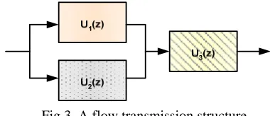
is strictly defined by the type of connection between elements in the reliability logic-diagram sense, i.e. on the structure of the logic-diagram representing the system/subsystem. Despite the fact that the universal generating function resembles a polynomial, it is not a [image:4.612.342.532.170.252.2]polynomial because: i.) its exponents are not necessary scalar variables, but can be arbitrary mathematical objects (e.g. vectors); ii.) operators defined over the universal generating function can differ from the operator of the polynomial product (unlike the ordinary generating function technique, only the product of polynomials is defined) [6].
Fig. 3 idealizes a general flow transmission through out the system (e.g., ore, fluid, energy)
Fig.3. A flow transmission structure
For instance, consider a flow transmission system shown in fig. 3 which consists of three elements. The system performance rate which is defined by its transmission capacity can have several discrete values depending on the state of control equipments.
The element 1 has three states with the performance rates
g11 = 1.5, g12 = 1, g13 = 0 and the corresponding probabilities
11
p
= 0.8,
p12= 0.1 and
p13= 0.1. The element 2 has three states with the performance rates g21 = 2, g22 = 1.5, g23 = 0 and the corresponding probabilities
p21= 0.7,
p22=0.22 and
p23= 0.08. The element 3 has two states with the performance rates g31 = 4, g32 = 0 and the corresponding probabilities
p31= 0.98 and
p32= 0.02. According to (9) the total number of the possible combinations of the states of elements is
p= 3 × 3 × 2 = 18.In order to obtain the output
pfor entire system with the arbitrary structure function
(.)
, [7] used a general composition operator
over individual universal z-transform representations of n system elements:
1 2
1 2
1
1
( ,.., )
1
( )
( ), ...,
( )
( )
.
( )
...
.
j
ji j j
n
jij nin
n
n k
g d ji i
k
k k n
g g d j
i i i j
U z
u z
u z
u z
z
U z
z
(11)
where
U z
( )
is z-transform representation of output performance distribution for the entire system.Consider
x x x
1,
2,
3,
y y
1,
2andy
3represent l,
r,n
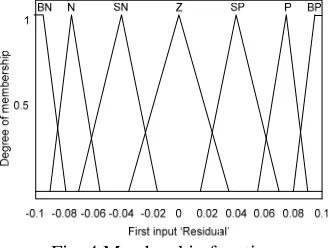
p, l [image:4.612.319.560.514.677.2][ 0.1, 0.1]
. The input and output linguistic variables adopted are Big Negative (BN), Negative (N), Small Negative (SN), Zero (Z), Small Positive (SP), Positive (P) and Big Positive (BP). Fig. 4 illustrates the membership functions.Fig. 4 Membership functions
Despite the operator expertise and knowledge at the level of the inference rules and the membership functions, some defects may appear. The degree of membership of each value of attribute
i
kin any of its fuzzy sets is directly based on the evaluation of the membership function of the particular fuzzy set with the value ofi
kas input. To improve the conventional FLC, association rules mining algorithms are used to find the optimal membership functions. This is achieved according to the following stages.B. Association rules Miming Algorithm
Specified fuzzy linguistic terms in fuzzy association rules can be given only when the properties of the attributes are estimated. In real life, contents of columns (i.e., values of attributes) may be unknown and meaningful intervals are usually not concise and crisp enough. In this paper, the target is to find out some interesting and potentially useful regularities, i.e., fuzzy association rules with enough support and high confidence. We use the following form for fuzzy association rules.
Let be
x
i1, ...,
x
ik
and
y
1i, ...,
y
ik
the antecedent set and the consequence set respectively, in a database. A fuzzy association rule mining is expressed as:If
X
x
i1, ...,
x
ik
isA
i1, ...,
ik
ThenY
y
i1, ...,
y
ik
isB
i1, ...,
ik
Here, X and Y are disjoint sets of attributes called item-sets, i.e.,
X
I
;Y
I
andX
Y
. A and Bcontain the fuzzy sets associated with corresponding attributes in X and Y, respectively.
Let
(.)
represent the membership value of each element of the antecedent and the consequence set.Under fuzzy taxonomies, using the measurements could result in some mistakes. Consider for instance the two following conditions:
1-
(
x
ik)
(
y
ik)
and
(
x
ik)
(
y
im)
2-(
k)
(
k)
i i
x
y
and(
k)
(
m)
i i
x
y
In the first condition, the confidence under fuzzy taxonomies of the two rules is equal, while in the second, the coverage of the two rules is equal. This situation rise the following question: which rule can be judged as best evidence rule?
For a rule to be interesting, it should have enough support and high confidence value, larger than user specified thresholds. To generate fuzzy association rules, all sets of items that have a support above a user specified threshold should be determined first. Item-sets with at least a minimum support are called frequent or large item-sets.
In the proposed method the algorithm iterations alternate between the generation of the candidate and frequent item-sets until large item-item-sets are identified. The fuzzy support value of item-set Z is calculated as:
(
, ( ))
( , )
t Ti zj Z j i jT
F t z
S Z F
n
(12)where
n
Tis the number of transactions in the database. Also, to ensure the accuracy of rules base, the consequent strength measure,
is used to estimate the mined rules as:1 1 1 1 1
( ) ( ) ( )
X Y Y
k k k
n n
k m j
i i i
i k m i j
y y y
(13)IV. SIMULATION RESULTS
Through available actuators it is possible to adjust the speed of the grinding circuit feeders, the fluid added to the mill and sump, the pump and the driving motor speed. The level of the sump is controlled by adjusting the set-point of pump velocity.
0 5 10 15 20 25 30 35 40 45 -12
-10 -8 -6 -4 -2 0 2x 10
-4
Time [s]
Outputs
Y1
[image:6.612.87.265.71.233.2]Y2
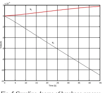
Fig. 5 Coupling degree of breakage process
Fig.5 illustrates coupling phenomena that exists between the controller variables (e.g., the entrance of negative pressure and the motor rotation speed).
0 5 10 15 20 25 30 35 40 45
0 0.2 0.4 0.6 0.8 1 1.2 1.4
time [s]
Ou
tp
u
ts
[image:6.612.74.278.288.450.2]
Fig. 6 Fuzzy Logic Controller step response
Using the aforementioned fuzzy logic rules the simulated step response of the grinding circuit is shown in fig.6. As shown in fig.6, in the presence of disturbances the fuzzy logic controller model presents a response better than the conventional PID model.
CONCLUSION
Simulation results show that the association rules mining algorithm is a feasible control rules generation algorithm to the fuzzy logic controller. Obviously it can be deduced that the fuzzy controller is faster than the conventional controller in the transitional state, and presents also a much smoother signal with less fluctuations in steady state. The proposed method can overcome nonlinear and strong coupling features of mineral processing in a wide range. It has strong robustness and adaptability.
REFERENCE
[1.] Abou S.C., “Contribution to ball mill modeling”. Doctorate thesis, Laval University, Ca. 1998.
[2.] Agrawal R., Imielinski T., and Swami A. “Mining association rules between sets of items in large databases. Int. Conf. on Management of Data (ACM SIGMOD ’93, Washington, 1993 [3.] Davis, E.W., Fine crushing in ball mills. AIME Transaction,
vol. 61, pp250-296. 1919
[4.] Desbiens A., K. Najim, A. Pomerleau and D. Hodouin,
“Adaptive control-practical aspects and application to a
grinding circuit,” Optim. Control Appl. Methods, vol. 18, pp.
29-47, 1997
[5.] Guan J., Wu Y., “Repairable consecutive-k-out-of-n: F system with fuzzy states”. Fuzzy Sets and Systems, vol.157 pp.121-142, 2006
[6.] Huang J., Zuo M.J., Wu Y., “Generalized multi-state k-out-of-n: G systems”, IEEE Trans. Reliability vol.49, no.1, pp.105-111, 2000
[7.] Kuo W., Wan R., “Recent advances in optimal reliability allocation”, IEEE Trans. Systems, Man Cybernet. Part A: Systems Humans, vol.37, pp.143-156, 2007
[8.] Levitin G., “Universal Generating Function and its Applications”, Springer, Berlin, 2005
[9.] Morell S., The prediction of powder draws in wet tumbling mills. Doctorate thesis, University of Queensland1993 [10.]Rajamani R.K. and J.A. Herbst, “Optimal control of a ball mill
grinding circuit: II. Feedback and optimal control” Chem. Eng.
Sci. vol.46, no.3, pp. 871-879, 1991
[11.]Weller K. R, “Automation in mining, mineral and metal processing”, Proc. 3rd IFAC symposium Pergamon Press. pp. 295-302, 1980.
[12.]Zhai Lianfei, and Chai Tianyou. “Nonlinear decoupling PID control using neural networks and multiple models,” J. of Control Theory and Applications, vol.4, no.1, pp. 62-69, 2006 [13.]Zimmermann H.J., “Fuzzy Set Theory and its Application,” 2nd