A Unified Model for Word Sense Representation and Disambiguation

A Unified Model for Word Sense Representation and Disambiguation

Xinxiong Chen, Zhiyuan Liu, Maosong Sun

State Key Laboratory of Intelligent Technology and Systems Tsinghua National Laboratory for Information Science and Technology

Department of Computer Science and Technology Tsinghua University, Beijing 100084, China

[email protected], {lzy, sms}@tsinghua.edu.cn

Abstract

Most word representation methods assume that each word owns a single semantic vec-tor. This is usually problematic because lexical ambiguity is ubiquitous, which is also the problem to be resolved by word sense disambiguation. In this paper, we present a unified model for joint word sense representation and disambiguation, which will assign distinct representation-s for each word representation-senrepresentation-se.1 _{The basic idea is} that both word sense representation R) and word sense disambiguation (WS-D) will benefit from each other: (1) high-quality WSR will capture rich informa-tion about words and senses, which should be helpful for WSD, and (2) high-quality WSD will provide reliable disambiguat-ed corpora for learning better sense rep-resentations. Experimental results show that, our model improves the performance of contextual word similarity compared to existing WSR methods, outperforms state-of-the-art supervised methods on domain-specific WSD, and achieves competitive performance on coarse-grained all-words WSD.

1 Introduction

Word representation aims to build vectors for each word based on its context in a large corpus, usually capturing both semantic and syntactic information of words. These representations can be used as features or inputs, which are widely employed in information retrieval (Manning et al., 2008), doc-ument classification (Sebastiani, 2002) and other NLP tasks.

1_{Our sense representations can be downloaded athttp:} //pan.baidu.com/s/1eQcPK8i.

Most word representation methods assume each word owns a single vector. However, this is usual-ly problematic due to the homonymy and pousual-lyse- polyse-my of many words. To remedy the issue, Reisinger and Mooney (2010) proposed a multi-prototype vector space model, where the contexts of each word are first clustered into groups, and then each cluster generates a distinct prototype vector for a word by averaging over all context vectors with-in the cluster. Huang et al. (2012) followed this idea, but introduced continuous distributed vectors based on probabilistic neural language models for word representations.

These cluster-based models conduct unsuper-vised word sense induction by clustering word contexts and, thus, suffer from the following is-sues:

• It is usually difficult for these cluster-based models to determine the number of cluster-s. Huang et al. (2012) simply cluster word contexts into staticKclusters for each word, which is arbitrary and may introduce mis-takes.

• These cluster-based models are typically off-line , so they cannot be efficiently adapted to new senses, new words or new data.

• It is also troublesome to find the sense that a word prototype corresponds to; thus, these cluster-based models cannot be directly used to perform word sense disambiguation. In reality, many large knowledge bases have been constructed with word senses available online, such as WordNet (Miller, 1995) and Wikipedia. Utilizing these knowledge bases to learn word representation and sense representation is a natural choice. In this paper, we present a uni-fied model for both word sense representation and disambiguation based on these knowledge bases and large-scale text corpora. The unified model

can (1) perform word sense disambiguation based on vector representations, and (2) learn continu-ous distributed vector representation for word and sense jointly.

The basic idea is that, the tasks of word sense representation (WSR) and word sense disam-biguation (WSD) can benefit from each other: (1) high-quality WSR will capture rich semantic and syntactic information of words and senses, which should be helpful for WSD; (2) high-quality WS-D will provide reliable disambiguated corpora for learning better sense representations.

By utilizing these knowledge bases, the prob-lem mentioned above can be overcome:

• The number of senses of a word can be de-cided by the expert annotators or web users.

• When a new sense appears, our model can be easily applied to obtain a new sense represen-tation.

• Every sense vector has a corresponding sense in these knowledge bases.

We conduct experiments to investigate the per-formance of our model for both WSR and WS-D. We evaluate the performance of WSR using a contextual word similarity task, and results show that out model can significantly improve the cor-relation with human judgments compared to base-lines. We further evaluate the performance on both domain-specific WSD and coarse-grained all-words WSD, and results show that our model yields performance competitive with state-of-the-art supervised approaches.

2 Methodology

We describe our method as a 3-stage process:

1. Initializing word vectors and sense vectors. Given large amounts of text data, we first use the Skip-gram model (Mikolov et al., 2013), a neural network based language model, to learn word vectors. Then, we assign vector representations for senses based on their def-initions (e.g, glosses in WordNet).

2. Performing word sense disambiguation. Given word vectors and sense vectors, we propose two simple and efficient WSD algo-rithms to obtain more relevant occurrences for each sense.

3. Learning sense vectors from relevant oc-currences. Based on the relevant occur-rences of ambiguous words, we modify the training objective of Skip-gram to learn word vectors and sense vectors jointly. Then, we obtain the sense vectors directly from the model.

Before illustrating the three stages of our method in Sections 2.2, 2.3 and 2.4, we briefly introduce our sense inventory, WordNet, in Sec-tion 2.1. Note that, although our experiments will use the WordNet sense inventory, our model is not limited to this particular lexicon. Other knowledge bases containing word sense distinctions and defi-nitions can also serve as input to our model.

2.1 WordNet

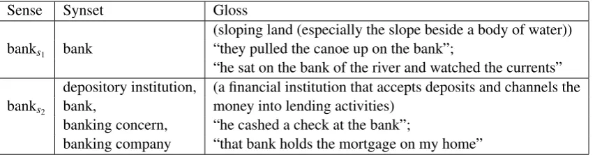
WordNet (Miller, 1995) is the most widely used computational lexicon of English where a concep-t is represenconcep-ted as a synonym seconcep-t, orsynset. The words in the same synset share a common mean-ing. Each synset has a textual definition, or gloss. Table 1 shows the synsets and the corresponding glosses of the two common senses ofbank.

Before introducing the method in detail, we in-troduce the notations. The unlabeled texts are de-noted asR, and the vocabulary of the texts is de-noted asW. For a word w inW, wsi is the ith sense in WordNetWN. Each sensewsi has a gloss

gloss(wsi) inWN. The word embedding of wis

denoted asvec(w), and the sense embedding of its ith sensewsi is denoted asvec(wsi).

2.2 Initializing Word Vectors and Sense Vectors

Initializing word vectors. First, we use Skip-gram to train the word vectors from large amounts of text data. We choose Skip-gram for its sim-plicity and effectiveness. The training objective of Skip-gram is to train word vector representations that are good at predicting its context in the same sentence (Mikolov et al., 2013).

More formally, given a sequence of training words w1, w2, w3,...,wT, the objective of Skip-gram is to maximize the average log probability

1 T

T

∑

t=1 −k≤

∑

!

(1)

Sense Synset Gloss

banks1

(sloping land (especially the slope beside a body of water)) bank “they pulled the canoe up on the bank”;

“he sat on the bank of the river and watched the currents”

banks2

depository institution, (a financial institution that accepts deposits and channels the bank, money into lending activities)

banking concern, “he cashed a check at the bank”;

banking company “that bank holds the mortgage on my home”

Table 1: Example of a synset in WordNet.

the log probability of correctly predicting the word wt+j given the word in the middlewt. The outer summation covers all words in the training data.

The prediction task is performed via softmax, a multiclass classifier. There, we have

p(wt+j|wt) = exp(vec

0_(wt+j)>_vec(w

t))

∑W_w=1exp(vec0_(w)>_vec(wt)) (2)

where vec(w) and vec0_{(w) are the “input” and}

“output” vector representations ofw. This formu-lation is impractical because the cost of comput-ingp(wt+j|wt)is proportional toW, which is often large( 105₋₁₀7_terms).

Initializing sense vectors. After learning the word vectors using the Skip-gram model, we ini-tialize the sense vectors based on the glosses of senses. The basic idea of the sense vector initial-ization is to represent the sense by using the sim-ilar words in the gloss. From the content words in the gloss, we select those words whose cosine similarities with the original word are larger than a similarity thresholdδ. Formally, for each sense wsi in WN, we first define a candidate set from gloss(wsi)

cand(wsi) ={u|u∈gloss(wsi),u6=w,

POS(u)∈CW,cos(vec(w),vec(u))>δ} (3)

wherePOS(u)is the part-of-speech tagging of the word uandCW is the set of all possible part-of-speech tags that content words could have. In this paper,CW contains the following tags: noun, verb, adjective and adverb.

Then the average of the word vectors in cand(wsi)is used as the initialization value of the sense vectorvec(wsi).

vec(wsi) = 1

|cand(wsi)|_u∈cand

∑

vec(u) (4)

For example, in WordNet, the gloss of the sense banks1 is “sloping land (especially the slope beside

a body of water)) they pulled the canoe up on the bank; he sat on the bank of the river and watched the currents”. The gloss contains a definition of the sense and two examples of the sense. The content words and the cosine similarities with the word “bank” are listed as follows: (sloping, 0.12), (land, 0.21), (slope, 0.17), (body, 0.01), (water, 0.10), (pulled, 0.01), (canoe, 0.09), (sat, 0.06), (river, 0.43), (watch, -0.11), (currents, 0.01). If the threshold,δ, is set to 0.05, then cand(banks1)

is {sloping, land, slope, water, canoe, sat, riv-er}. Then the average of the word vectors in cand(banksi) is used as the initialization value of vec(banksi).

2.3 Performing Word Sense Disambiguation. One of the state-of-the-art WSD results can be obtained using exemplar models, i.e., the word meaning is modeled by using relevant occurrences only, rather than merging all of the occurrences in-to a single word vecin-tor (Erk and Pado, 2010). In-spired by this idea, we perform word sense disam-biguation to obtain more relevant occurrences.

Here, we perform knowledge-based word sense disambiguation for training data on an all-words setting, i.e., we will disambiguate all of the con-tent words in a sentence. Formally, the sentenceS is a sequence of words (w1,w2,...,wn), and we will identify a mappingMfrom words to senses such thatM(i)∈SensesWN(wi), whereSensesWN(wi)is the set of senses encoded in theWNfor wordwi. For sentenceS, there are∏ni=1|SenseWN(wi)| pos-sible mapping answers, which are impractical to compute. Thus, we design two simple algorithms, L2R (left to right) algorithm and S2C (simple to complex) algorithm, for word sense disambigua-tion based on the sense vectors.

the order of words when performing word sense disambiguation. When given a sentence, the L2R algorithm disambiguates the words from left to right (the natural order of a sentence), whereas the S2C algorithm disambiguates the words with few-er senses first. The main idea of S2C algorithm is that the words with fewer senses are easier to disambiguate, and the disambiguation result can be helpful to disambiguate the words with more senses. Both of the algorithms have three steps: Context vector initialization. Similar to the ini-tialization of sense vectors, we use the average of all of the content words’ vectors in a sentence as the initialization vector of context.

vec(context) = 1

|cand(S)|_u∈cand

∑

where cand(S) is the set of content words cand(S) ={u|u∈S,POS(u)∈CW}.

Ranking words. For L2R, we do nothing in this step. For S2C, we rank the words based on the ascending order of|SensesWN(wi)|.

Word sense disambiguation. For both L2R and S2C, we denote the order of words asL and per-form word sense disambiguation according toL.

First, we skip a word if the word is not a content word or the word is monosemous (|SensesWN(wi)|=1). Then, for each word in L, we can compute the cosine similarities be-tween the context vector and its sense vectors. We choose the sense that yields the maximum cosine similarity as its disambiguation result. If the s-core margin between the maximum and the sec-ond maximum is larger than the thresholdε, we are confident with the disambiguation result ofwi and then use the sense vector to replace the word vector in the context vector. Thus, we obtain a more accurate context vector for other words that are still yet to be disambiguated.

For example, given a sentence “He sat on the bank of the lake”, we first explain how S2C work-s. In the sentence, there are three content word-s, “sat”, “bank” and “lake”, to be disambiguated. First, the sum of the three word vectors is used as the initialization of the context vector. Then we rank the words by |SensesWN(wi)|, in ascending order, that is, lake (3 senses), bank (10 senses), sat (10 senses). We first disambiguate the word “lake” based on the similarities between its sense vectors and context vector. If the score margin is larger

bank input

projection output

sat sit₁ on the of the lakelake₁

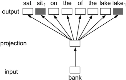
Figure 1: The architecture of our model. The training objective of Skip-gram is to train word vector representations that are not only good at predicting its context words but are also good at predicting its context words’ senses. The center word “bank” is used to predict not only its context words but also the sense “sit1” and “lake1”.

than the threshold ε, then we are confident with this disambiguation result and replace the word vector with the sense vector to update the contex-t veccontex-tor. Icontex-t would be helpful contex-to disambiguacontex-te contex-the next word, “bank”. We repeat this process until all three words are disambiguated.

For L2R, the order of words to be disambiguat-ed will be “sat”, “bank” and “lake”. In this time, when disambiguating “bank” (10 senses), we still don’t know the sense of “lake” (3 senses).

2.4 Learning Sense Vectors from Relevant Occurrences.

Based on the disambiguation result, we modify the training objective of Skip-gram and train the sense vectors directly from the large-scale corpus. Our training objective is to train the vector representa-tions that are not only good at predicting its text words but are also good at predicting its con-text words’ senses. The architecture of our model is shown in Figure 1.

More formally, given the disambiguation result M(w1),M(w2),M(w3),...,M(wT), the training ob-jective is modified to

1 T

T

∑

t=1 k

∑

j=−klog{p(wt+j|wt)p(M(wt+j)|wt)}

!

the sense M(wt+j) given the word in the middle wt. The outer summation covers all words in the training data.

Because not all of the disambiguation results are correct, we only disambiguate the words that we are confident in. Similar to step 3 of our WSD algorithm, we only disambiguate words under the condition that the score margin between the max-imum and the second maxmax-imum is larger than the score margin threshold,ε.

We also use the softmax function to define p(wt+j|wt)and p(M(wt+j)|wt). Then, we use hi-erarchical softmax (Morin and Bengio, 2005) to greatly reduce the computational complexity and learn the sense vectors directly from the relevant occurrences.

3 Experiments

In this section, we first present the nearest neigh-bors of some words and their senses, showing that our sense vectors can capture the semantics of words. Then, we use three tasks to evaluate our u-nified model: a contextual word similarity task to evaluate our sense representations, and two stan-dard WSD tasks to evaluate our knowledge-based WSD algorithm based on the sense vectors. Ex-perimental results show that our model not only improves the correlation with human judgments on the contextual word similarity task but also out-performs state-of-the-art supervised WSD system-s on domain-system-specific datasystem-setsystem-s and competesystem-s with them in a coarse-grained all-words setting.

We choose Wikipedia as the corpus to train the word vectors because of its wide coverage of topics and words usages. We use an English Wikipedia database dump from October 2013 2_, which includes roughly 3 million articles and 1 billion tokens. We use Wikipedia Extractor 3 _to preprocess the Wikipedia pages and only save the content of the articles.

We use word2vec4_{to train Skip-gram. We use} the default parameters of word2vec and the dimen-sion of the vector representations is 200.

We use WordNet5 _{as our sense inventory. The} datasets for different tasks are tagged with differ-ent versions of WordNet. The version of WordNet

2_{http://download.wikipedia.org.}

3_{The tool is available fromhttp://medialab.di.} unipi.it/wiki/Wikipedia_Extractor.

4_{The code is available from https://code.} google.com/p/word2vec/.

5_{http://wordnet.princeton.edu/.}

Word or sense Nearest neighbors bank banks, IDBI, CitiBank

banks1 river, slope, Sooes

banks2 mortgage, lending, loans

star stars, stellar, trek stars1 photosphere, radiation,_gamma-rays

stars2 someone, skilled, genuinely

plant plants, glavaticevo, herbaceous plant_s1 factories, machinery,_{manufacturing}

plant_s2 locomotion, organism,_organisms

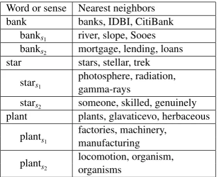
Table 2: Nearest neighbors of word vectors and sense vectors learned by our model based on co-sine similarity. The subscript of each sense label corresponds to the index of the sense in Word-Net. For example, banks2 is the second sense of

the word bank in WordNet.

is 1.7 for the domain-specific WSD task and 2.1 for the coarse-grained WSD task.

We use the S2C algorithm described in Section 2.3 to perform word sense disambiguation to ob-tain more relevant occurrences for each sense. We compare S2C and L2R on the coarse-grained WS-D task in a all-words setting.

The experimental results of our model are ob-tained by setting the similarity threshold asδ =0 and the score margin threshold asε=0.1. The in-fluence of parameters on our model can be found in Section 3.5.

3.1 Examples for Sense Vectors

Table 2 shows the nearest neighbors of word vec-tors and sense vecvec-tors based on cosine similarty. We see that our sense representations can i-dentify different meanings of a word, allowing our model to capture more semantic and syntactic re-lationships between words and senses. Note that each sense vector in our model corresponds to a sense in WordNet; thus, our sense vectors can be used to perform knowledge-based word sense dis-ambiguation, whereas the vectors of cluster-based models cannot.

3.2 Contextual Word Similarity

con-Model ρ×100

C&W-S 57.0

Huang-S 58.6

Huang-M AvgSim 62.8

Huang-M AvgSimC 65.7

Our Model-S 64.2

Our Model-M AvgSim 66.2 Our Model-M AvgSimC 68.9

Table 3: Spearman’sρon the SCWS dataset. Our Model-S uses one representation per word to com-pute similarities, while Our Model-M uses one representation per sense to compute similarities. AvgSim calculates the similarity with each sense contributing equally, while AvgSimC weighs the sense according to the probability of the word choosing that sense in contextc.

sists of 353 pairs of nouns. However, each pair of nouns in WordSim-353 is presented without con-text. This is problematic because the meanings of homonymous and polysemous words depend highly on the words’ contexts. Thus we choose the Stanford’s Contextual Word Similarities (SCWS) dataset from (Huang et al., 2012) 6_{. The SCWS} dataset contains 2003 pairs of words and each pair is associated with 10 human judgments on similar-ity on a scale from 0 to 10. In the SCWS dataset, each word in a pair has a sentential context.

In our experiments, the similarity between a pair of words (w,w0_{) is computed as follows:}

AvgSimC(w,w0_{) =} 1

MN M

∑

i=1 N

∑

j=1 p(i|w,c)p(j|w0_,c0_)d(vec(ws

i),vec(w0sj)) (7) where p(i|w,c) is the likelihood that word w chooses itsith sense given contextc. d(vec,vec0₎

is a function computing the similarity between two vectors, and here we use cosine similarity.

Results and discussion. For evaluation, we compute the Spearman correlation between a model’s computed similarity scores and human judgements. Table 3 shows our results com-pared to previous methods, including (Collobert and Weston, 2008)’s language model (C&W), and Huang’s model which utilize the global context and multi-prototype to improve the word represen-tations.

6_{The dataset can be downloaded at http://ai.} stanford.edu/˜ehhuang/.

From Table 3, we observe that:

• Our single-vector version outperforms Huang’s single-vector version. This indi-cates that, by training the word vectors and sense vectors jointly, our model can better capture the semantic relationships between words and senses.

• With one representation per sense, our mod-el can outperform the single-vector version without using context (66.2 vs. 64.2).

• Our model obtains the best performance (68.9) by using AvgSimC, which takes con-text into account.

3.3 Domain-Specific WSD

Experimental setting. We use Wikipedia as training data because of its wide coverage for spe-cific domains. To test our performance on do-main word sense disambiguation, we evaluated our system on the dataset published in (Koeling et al., 2005). This dataset consists of examples retrieved from the Sports and Finance sections of the Reuters corpus. 41 words related to the Sports and Finance domains were selected, with an aver-age polysemy of 6.7 senses, ranging from 2 to 13 senses.

Approximately 100 examples for each word were annotated with senses from WordNet v.1.7 by three reviewers, yielding an inter-tagger agree-ment of 65%. (Koeling et al., 2005) did not clarify how to select the “correct” sense for each word, so we followed the work of (Agirre et al., 2009) and, used the sense chosen by the majority of taggers as the correct answer.

Baseline methods. As a baseline, we use the most frequent WordNet sense (MFS), as well as a random sense assignment. We also compare our results with four systems7_{: Static PageRank} (A-girre et al., 2009), theknearest neighbor algorith-m (k-NN), Degree (Navigli and Lapata, 2010) and Personalized PageRank (Agirre et al., 2009).

Static PageRank applies traditional PageRank over the semantic graph based on WordNet and obtains a context-independent ranking of word senses.

k-NN is a widely used classification method, where neighbors are thek labeled examples most

7_{We compare only with those systems performing}

Algorithm Sports Finance_{Recall Recall} Random BL 19.5 19.6

MFS BL 19.6 37.1

k-NN 30.3 43.4

Static PR 20.1 39.6 Personalized PR 35.6 46.9

Degree 42.0 47.8

Our Model 57.3 60.6

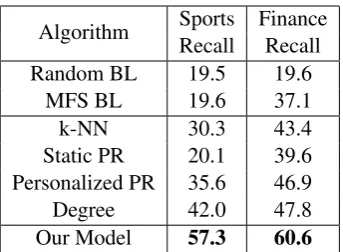
Table 4: Performance on the Sports and Finance sections of the dataset from (Koeling et al., 2005).

similar to the test example. Thek-NN system is trained on SemCor (Miller et al., 1993), the largest publicly available annotated corpus.

Degree and Personalized PageRank are state-of-the-art systems that exploit WordNet to build a semantic graph and exploit the structural proper-ties of the graph in order to choose the appropriate senses of words in context.

Results and discussion. Similar to other work on this dataset, we use recall (the ratio of correct sense labels to the total labels in the gold standard) as our evaluation measure. Table 4 shows the re-sults of different WSD systems on the dataset, and the best results are shown in bold. The differences between other results and the best result in each column of the table are statistically significant at p<0.05.

The results show that:

• Our model outperforms k-NN on the t-wo domains by a large margin, support-ing the findsupport-ings from (Agirre et al., 2009) that knowledge-based systems perform bet-ter than supervised systems when evaluated across different domains.

• Our model also achieves better results than the state-of-the-art system (+15.3% recall on Sports and +12.8% recall on Finance against Degree). The reason for this is that when dealing with short sentences or context words that are not in WordNet, our model can still compute similarity based on the context vec-tor and sense vecvec-tors, whereas Degree will have difficulty building the semantic graph.

• Moreover, our model achieves the best per-formance by only using the unlabeled text da-ta and the definitions of senses, whereas other

Algorithm Type Nouns only All words_F

1 F1

Random BL U 63.5 62.7

MFS BL Semi 77.4 78.9

SUSSX-FR Semi 81.1 77.0

NUS-PT S 82.3 82.5

SSI Semi 84.1 83.2

Degree Semi 85.5 81.7

Our ModelL2R U 79.2 73.9 Our ModelS2C U 81.6 75.8 Our ModelL2R Semi 82.5 79.6 Our ModelS2C Semi 85.3 82.6

Table 5: Performance on Semeval-2007 coarse-grained all-words WSD. In the type column, U, Semi and S stand for unsupervised, semi-supervised and semi-supervised, respectively. The dif-ferences between the results in bold in each col-umn of the table are not statistically significant at p<0.05.

methods rely greatly on high-quality seman-tic relations or annotated data, which are hard to acquire.

3.4 Coarse-grained WSD

Experimental setting. We also evaluate our WSD model on the Semeval-2007 coarse-grained all-words WSD task (Navigli et al., 2007). There are multiple reasons that we perform experiments in a coarse-grained setting: first, it has been ar-gued that the fine granularity of WordNet is one of the main obstacles to accurate WSD (cf. the discussion in (Navigli, 2009)); second, the train-ing corpus of word representations is Wikipedia, which is quite different from WordNet.

Results and discussion. We report our results in terms of F1-measure on the Semeval-2007 coarse-grained all-words dataset (Navigli et al., 2007). Table 5 reports the results for nouns (1,108 words) and all words (2,269 words). The difference be-tween unsupervised and semi-supervised methods is whether the method uses MFS as a back-off s-trategy.

We can see that the S2C algorithm outperforms the L2R algorithm no matter on the nouns subset or on the entire set. This indicates that words with fewer senses are easier to disambiguate, and it can be helpful to disambiguate the words with more senses.

On the nouns subset, our model yields compa-rable performance to SSI and Degree, and it out-performs NUS-PT and SUSSX-FR. Moreover, our unsupervised WSD method (S2C) beats the MF-S baseline, which is notably a difficult competitor for knowledge-based systems.

On the entire set, our semi-supervised model is significantly better than SUSSX-FR, and it is com-parable with SSI and Degree. In contrast to SSI, our model is simple and does not rely on a cost-ly annotation effort to engineer the set of semantic relations.

Overall, our model achieves state-of-the-art per-formance on the Semeval-2007 coarse-grained all-words dataset compared to other systems, with a simple WSD algorithm that only relies on a large-scale unlabeled text corpora and a sense inventory.

3.5 Parameter Influence

We investigate the influence of parameters on our model with coarse-grained all-words WSD task. The parameters include the similarity threshold,δ, and the score margin threshold,ε.

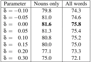
Similarity threshold. In Table 6, we show the performance of domain WSD when the similari-ty thresholdδ ranges from−0.1 to 0.3. The co-sine similarity interval is [-1, 1], and we focus on the performance in the interval [-0.1, 0.3] for two reasons: first, no words are removed from glosses whenδ <−0.1; second, nearly half of the word-s are removed whenδ >0.3 and the performance drops significantly for the WSD task. From table 6, we can see that our model achieves the best per-formance whenδ =0.0.

Score margin threshold. In Table 7, we show the performance on the coarse-grained all-words

Parameter Nouns only All words δ =−0.10 79.8 74.3 δ =−0.05 81.0 74.6 δ = 0.00 81.6 75.8 δ = 0.05 81.3 75.4 δ = 0.10 80.8 75.2 δ = 0.15 80.0 75.0 δ = 0.20 77.1 73.3 δ = 0.30 75.0 72.1

Table 6: Evaluation results on the coarse-grained all-words WSD when the similarity threshold δ ranges from−0.1 to 0.3.

Parameter Nouns only All words ε=0.00 78.2 72.9 ε=0.05 79.5 74.5 ε=0.10 81.6 75.8 ε=0.15 81.2 74.7 ε=0.20 80.9 75.1 ε=0.25 80.2 74.8 ε=0.30 80.4 74.9

Table 7: Evaluation results on the coarse-grained all-words WSD when the score margin threshold ε ranges from 0.0 to 0.3.

WSD when the score margin threshold ε ranges from 0.0 to 0.3. When ε =0.0, we use every disambiguation result to update the context vec-tor. Whenε6=0, we only use the confident disam-biguation results to update the context vector if the score margin is larger thanε. Our model achieves the best performance whenε=0.1.

4 Related Work

4.1 Word Representations

(Li-u et al., 2010; Li(Li-u et al., 2011b; Li(Li-u et al., 2012), social tag suggestion (Liu et al., 2011a) and text classification (Baker and McCallum, 1998), may also potentially benefit from distributed word resentation. The main advantage is that the rep-resentations of similar words are close in vector space, which makes generalization to novel pat-terns easier and model estimation more robust.

Word representations are hard to train due to the computational complexity. Recently, (Mikolov et al., 2013) proposed two particular models, Skip-gram and CBOW, to learn word representations in large amounts of text data. The training objective of the CBOW model is to combine the representa-tions of the surrounding words to predict the word in the middle, while the Skip-gram model’s is to learn word representations that are good at predict-ing its context in the same sentence (Mikolov et al., 2013). Our paper uses the model architecture of Skip-gram.

Most of the previous vector-space models use one representation per word. This is problematic because many words have multiple senses. The multi-prototype approach has been widely stud-ied. (Reisinger and Mooney, 2010) proposed the multi-prototype vector-space model. (Huang et al., 2012) used the multi-prototype models to learn the vector for different senses of a word. All of these models use the clustering of contexts as a word sense and can not be directly used in word sense disambiguation.

After our paper was submitted, we perceive the following recent advances: (Tian et al., 2014) pro-posed a probabilistic model for multi-prototype word representation. (Guo et al., 2014) explored bilingual resources to learn sense-specific word representation. (Neelakantan et al., 2014) pro-posed an efficient non-parametric model for multi-prototype word representation.

4.2 Knowledge-based WSD

The objective of word sense disambiguation (WS-D) is to computationally identify the meaning of words in context (Navigli, 2009). There are t-wo approaches of WSD that assign meaning of words from a fixed sense inventory, supervised and knowledge-based methods. Supervised approach-es require large labeled training sets, which are time consuming to create. In this paper, we on-ly focus on knowledge-based word sense disam-biguation.

Knowledge-based approaches exploit knowl-edge resources (such as dictionaries, thesauri, on-tologies, collocations, etc.) to determine the senses of words in context. However, it has been shown in (Cuadros and Rigau, 2006) that the amount of lexical and semantic information contained in such resources is typically insuf-ficient for high-performance WSD. Much work has been presented to automatically extend ex-isting resources, including automatically linking Wikipedia to WordNet to include full use of the first WordNet sense heuristic (Suchanek et al., 2008), a graph-based mapping of Wikipedia cat-egories to WordNet synsets (Ponzetto and Nav-igli, 2009), and automatically mapping Wikipedia pages to WordNet synsets (Ponzetto and Navigli, 2010).

It was recently shown that word representation-s can capture representation-semantic and representation-syntactic information between words (Mikolov et al., 2013). Some re-searchers tried to incorporate WordNet senses in a neural model to learn better word representation-s (Borderepresentation-s et al., 2011). In thirepresentation-s paper, we have pro-posed a unified method for word sense representa-tion and disambiguarepresenta-tion to extend the informarepresenta-tion contained in the vector representations to the ex-isting resources. Our method only requires a large amount of unlabeled text to train sense representa-tions and a dictionary to provide the definirepresenta-tions of word meanings, which makes it easily applicable to other resources.

5 Conclusion

In this paper, we present a unified model for word sense representation and disambiguation that us-es one reprus-esentation per sense. Experimental re-sults show that our model improves the perfor-mance of contextual word similarity compared to existing WSR methods, outperforms state-of-the-art supervised methods on domain-specific WSD, and achieves competitive performance on coarse-grained all-words WSD. Our model only requires large-scale unlabeled text corpora and a sense in-ventory for WSD, thus it can be easily applied to other corpora and tasks.

There are still several open problems that should be investigated further:

2. We can explore other WSD methods based on sense vectors to improve our performance. For example, (Li et al., 2010) used LDA to perform data-driven WSD in a manner simi-lar to our model. We may integrate the advan-tages of these models and our model together to build a more powerful WSD system. 3. To learn better sense vectors, we can exploit

the semantic relations (such as the hypernym and hyponym relations defined in WordNet) between senses in our model.

Acknowledgments

This work is supported by National Key Ba-sic Research Program of China (973 Program 2014CB340500) and National Natural Science Foundation of China (NSFC 61133012).

References

Eneko Agirre, Oier Lopez De Lacalle, Aitor Soroa, and Informatika Fakultatea. 2009. Knowledge-based wsd and specific domains: Performing better than

generic supervised wsd. InProceedings of IJCAI,

pages 1501–1506.

L Douglas Baker and Andrew Kachites McCallum. 1998. Distributional clustering of words for text

classification. In Proceedings of SIGIR, pages 96–

103.

Yoshua Bengio, Holger Schwenk, Jean-S´ebastien Sen´ecal, Fr´ederic Morin, and Jean-Luc Gauvain.

2006. Neural probabilistic language models. In

In-novations in Machine Learning, pages 137–186. Antoine Bordes, Jason Weston, Ronan Collobert,

Yoshua Bengio, et al. 2011. Learning structured

embeddings of knowledge bases. InProceedings of

AAAI, pages 301–306.

Yee Seng Chan, Hwee Tou Ng, and Zhi Zhong. 2007. Nus-pt: exploiting parallel texts for word sense

dis-ambiguation in the english all-words tasks. In

Pro-ceedings of SemEval, pages 253–256.

Ronan Collobert and Jason Weston. 2008. A unified architecture for natural language processing: Deep

neural networks with multitask learning. In

Pro-ceedings of ICML, pages 160–167.

Ronan Collobert, Jason Weston, L´eon Bottou, Michael Karlen, Koray Kavukcuoglu, and Pavel Kuksa. 2011. Natural language processing (almost) from

scratch. JMLR, 12:2493–2537.

Montse Cuadros and German Rigau. 2006. Quality assessment of large scale knowledge resources. In Proceedings of EMNLP, pages 534–541.

Katrin Erk and Sebastian Pado. 2010. Exemplar-based

models for word meaning in context. InProceedings

of ACL, pages 92–97.

Lev Finkelstein, Evgeniy Gabrilovich, Yossi Matias, E-hud Rivlin, Zach Solan, Gadi Wolfman, and Eytan Ruppin. 2001. Placing search in context: The

con-cept revisited. InProceedings of WWW, pages 406–

414.

Jiang Guo, Wanxiang Che, Haifeng Wang, and Ting Li-u. 2014. Learning sense-specific word embeddings

by exploiting bilingual resources. InProceedings of

COLING, pages 497–507.

Eric H Huang, Richard Socher, Christopher D Man-ning, and Andrew Y Ng. 2012. Improving word representations via global context and multiple word

prototypes. InProceedings of ACL, pages 873–882.

Rob Koeling and Diana McCarthy. 2007. Sussx: Ws-d using automatically acquireWs-d preWs-dominant senses. InProceedings of SemEval, pages 314–317.

Rob Koeling, Diana McCarthy, and John Carroll. 2005. Domain-specific sense distributions and

pre-dominant sense acquisition. InProceedings of

HLT-EMNLP, pages 419–426.

Linlin Li, Benjamin Roth, and Caroline Sporleder. 2010. Topic models for word sense disambiguation

and token-based idiom detection. InProceedings of

ACL, pages 1138–1147.

Zhiyuan Liu, Wenyi Huang, Yabin Zheng, and Maosong Sun. 2010. Automatic keyphrase

extrac-tion via topic decomposiextrac-tion. In Proceedings of

EMNLP, pages 366–376.

Zhiyuan Liu, Xinxiong Chen, and Maosong Sun. 2011a. A simple word trigger method for social tag

suggestion. InProceedings of EMNLP, pages 1577–

1588.

Zhiyuan Liu, Xinxiong Chen, Yabin Zheng, and Maosong Sun. 2011b. Automatic keyphrase

extrac-tion by bridging vocabulary gap. InProceedings of

CoNLL, pages 135–144.

Zhiyuan Liu, Xinxiong Chen, and Maosong Sun. 2012. Mining the interests of chinese microbloggers via

keyword extraction.Frontiers of Computer Science,

6(1):76–87.

Christopher D Manning, Prabhakar Raghavan, and

Hinrich Sch¨utze. 2008. Introduction to information

retrieval. Cambridge University Press Cambridge. Tomas Mikolov, Kai Chen, Greg Corrado, and Jeffrey

Dean. 2013. Efficient estimation of word

represen-tations in vector space.Proceedings of ICLR.

Tomas Mikolov. 2012. Statistical Language

George A Miller, Claudia Leacock, Randee Tengi, and Ross T Bunker. 1993. A semantic concordance. In Proceedings of the workshop on HLT, pages 303– 308.

George A Miller. 1995. Wordnet: a lexical

database for english. Communications of the ACM,

38(11):39–41.

Andriy Mnih and Geoffrey E Hinton. 2008. A s-calable hierarchical distributed language model. In Proceedings of NIPS, pages 1081–1088.

Frederic Morin and Yoshua Bengio. 2005. Hierarchi-cal probabilistic neural network language model. In Proceedings of the international workshop on artifi-cial intelligence and statistics, pages 246–252. Roberto Navigli and Mirella Lapata. 2010. An

ex-perimental study of graph connectivity for

unsu-pervised word sense disambiguation. IEEE PAMI,

32(4):678–692.

Roberto Navigli and Paola Velardi. 2005. Structural semantic interconnections: a knowledge-based

ap-proach to word sense disambiguation. IEEE PAMI,

27(7):1075–1086.

Roberto Navigli, Kenneth C Litkowski, and Orin Har-graves. 2007. Semeval-2007 task 07:

Coarse-grained english all-words task. In Proceedings of

SemEval, pages 30–35.

Roberto Navigli. 2009. Word sense disambiguation: A

survey. CSUR, 41(2):10.

Arvind Neelakantan, Jeevan Shankar, Alexandre Pas-sos, and Andrew McCallum. 2014. Efficient non-parametric estimation of multiple embeddings per

word in vector space. InProceedings of EMNLP.

Simone Paolo Ponzetto and Roberto Navigli. 2009. Large-scale taxonomy mapping for restructuring

and integrating wikipedia. InProceedings of IJCAI,

volume 9, pages 2083–2088.

Simone Paolo Ponzetto and Roberto Navigli. 2010. Knowledge-rich word sense disambiguation rivaling

supervised systems. InProceedings of ACL, pages

1522–1531.

Joseph Reisinger and Raymond J Mooney. 2010. Multi-prototype vector-space models of word

mean-ing. In Proceedings of HLT-NAACL, pages 109–

117.

David E Rumelhart, Geoffrey E Hintont, and Ronald J Williams. 1986. Learning representations by

back-propagating errors.Nature, 323(6088):533–536.

Fabrizio Sebastiani. 2002. Machine learning in

auto-mated text categorization. CSUR, 34(1):1–47.

Richard Socher, Cliff C Lin, Andrew Ng, and Chris Manning. 2011. Parsing natural scenes and natural

language with recursive neural networks. In

Pro-ceedings of ICML, pages 129–136.

Richard Socher, John Bauer, Christopher D Manning, and Andrew Y Ng. 2013. Parsing with

composi-tional vector grammars. InProceedings of ACL.

Fabian M Suchanek, Gjergji Kasneci, and Gerhard Weikum. 2008. Yago: A large ontology from

wikipedia and wordnet. Web Semantics:

Sci-ence, Services and Agents on the World Wide Web, 6(3):203–217.

Fei Tian, Hanjun Dai, Jiang Bian, Bin Gao, Rui Zhang, Enhong Chen, and Tie-Yan Liu. 2014. A probabilis-tic model for learning multi-prototype word

embed-dings. InProceedings of COLING, pages 151–160.

Joseph Turian, Lev Ratinov, and Yoshua Bengio. 2010. Word representations: a simple and general method

for semi-supervised learning. InProceedings of