L2 and Linfinity Stability Analysis of Heterogeneous Traffic With Application to Parameter Optimization for the Control of Automated Vehicles

See discussions, stats, and author profiles for this publication at: https://www.researchgate.net/publication/323818741

L

₂

_{and L}

∞

_{Stability Analysis of Heterogeneous Traffic With Application to}

Parameter Optimization for the Control of Automated Vehicles

Article  in  IEEE Transactions on Control Systems Technology · March 2018 DOI: 10.1109/TCST.2018.2808909

CITATIONS

2

READS

25

3 authors, including:

Douglas J. Leith

Trinity College Dublin

259 PUBLICATIONS   5,958 CITATIONS   

L

and

L

stability analysis of heterogeneous traffic

with application to parameter optimisation for the

control of automated vehicles

Julien Monteil1, M´elanie Bouroche2, Douglas J. Leith2

Abstract

The presence of (partially) automated vehicles on the roads presents an op-portunity to compensate the unstable behaviour of conventional vehicles. Vehicles subject to perturbations should (i) recover their equilibrium speed, (ii) react not to propagate but absorb perturbations. In this work, we start with considering vehicle systems consisting of heterogeneous vehicles updat-ing their dynamics accordupdat-ing to realistic behavioural car-followupdat-ing models. Definitions of all types of stability that are of interest in the vehicle system, namely input-output stability, scalability, weak and strict string stability, are introduced based on recent studies. Then, frequency domain linear stability analyses are conducted after linearisation of the modelled system of vehicles, leading to conditions for input-output stability, strict and weak string sta-bility over the behavioural parameters of the system, for finite and infinite systems of homogeneous and heterogeneous vehicles. This provides a solid basis that was missing for car-following model-based control design in mixed traffic systems where only a proportion of vehicles can be controlled. After visualisation of the theoretical results in simulation, we formulate an opti-misation strategy with LMI constraints to tune the behavioural parameters

of the automated vehicles in order to maximise the L∞ string stability of

the mixed traffic flow while considering the comfort of automated driving. The optimisation strategy systematically leads to increased traffic flow sta-bility. We show that very few automated vehicles are required to prevent the

1_{IBM Research - Ireland Lab, Control and Optimization Group. Address: Building 3,}

IBM Technology Campus, Mulhuddart, Dublin 15, Ireland.

2_{Trinity College Dublin - School of Computer Science. Address: College Green,}

propagation of realistic disturbances.

Keywords: L2 and L∞ stability analysis, L∞ string stability, Linear

Matrix Inequalities, automated vehicles, heterogeneous traffic.

1. Introduction

Interest is growing in how to control (partially) automated vehicles, i.e. vehicles equipped with Automated Driving Systems (ADS) such as Adap-tive Cruise Control (ACC), CooperaAdap-tive AdapAdap-tive Cruise Control (CACC), or any autopilot system, to increase traffic flow stability and safety in mixed traffic contexts, when (partially) automated vehicles and conventional vehi-cles coexist on the road. A recent report has underlined the unsafe nature of automated vehicles, which are five times more likely to crash than con-ventional vehicles, even though they are almost never to blame when a crash does occur Schoettle and Sivak (2015). In this context, one can assume that automated vehicles should behave similarly to surrounding drivers in order not to surprise them and, when automation is only partial, similarly to the in-vehicle driver in order to increase driving comfort and facilitate switch-ing between automated and conventional modes. As a result, the modellswitch-ing and understanding of conventional vehicles dynamics is particularly relevant for the design of driver-dependent, comfortable, and safe controllers for the acceleration dynamics of automated vehicles.

Regarding automated vehicle dynamics, a lot of attention has been put into the study of platoon systems, i.e. systems composed of automated vehi-cles that behave according to some distributed control protocol. Two stabil-ity objectives, namely stabilstabil-ity and string stabilstabil-ity, are commonly considered when designing distributed control protocols for some given communication topologies, see e.g. Knorn et al. (2014); Ploeg et al. (2014b). In particular, while stability characterises the convergence of the platooning system towards a desired equilibrium configuration, string stability refers to the attenuation of disturbances along the vehicle string. Note that, despite a number of early works Sheikholeslam and Desoer (1990, 1993); Zhou and Hui (2010); Naus et al. (2010), the lack of a unified definition for string stability was identified

in Ploeg et al. (2014b), where a definition ofLp string stability was proposed

Pro-gram Shladover et al. (1991); Varaiya and Shladover (1991). Among the contributions were the formulations of lateral and longitudinal control laws for stable, safe and comfortable platoon maneuvres, see Li et al. (1997); Frankel et al. (1996) for example, the development of a control system ar-chitecture for platooning, see Hedrick et al. (1994) for instance, and the San Diego demonstration in 1997 Tan et al. (1998). Since then, several linear con-trol protocols have been proposed over the years to address the stability and string stability of platoons, see e.g. Swaroop and Hedrick (1995); Liu et al. (2001). Very recently, the string stable behaviour of a linear CACC system

viaH∞ control was demonstrated Ploeg et al. (2014a), the stable platooning

of a linear control protocol considering communication delays was proved using the Lyapunov-Razumikhin theorem di Bernardo et al. (2015), a novel condition for the design of nonlinear control protocols for stable platooning was proposed Monteil and Russo (2017), and a protocol with nonlinear con-trol terms was proved to lead to string stable platooning via energy-based arguments Knorn et al. (2014).

the case of systems of heterogeneous vehicles, i.e. with vehicles exhibiting different car-following behaviour.

Contributions of the paper

in the context of the above literature, we propose a number of key novel-ties and contributions. First, we believe that the key and novel idea of this paper is that in mixed traffic environments (partially) automated vehicles can be used to compensate the string unstable behaviour of conventional vehi-cles. Differently to the problem of designing control protocols for automated platoon systems, here we focus on mixed vehicle systems where the dynam-ics of conventional vehicles are heterogeneous, follow realistic car-following behaviour and cannot be controlled. Furthermore, we work with the hy-pothesis that the automated vehicles should behave in a similar way to the conventional vehicles to maximise driving comfort and compliance with the automated system, and to minimise the occurrences of unusual behaviour. In such a context, the contributions in comparison with existing works are as follows: (i) we formalise the definition of weak stability that is relevant in mixed traffic environments made of automated and conventional vehicles; (ii) we investigate the stability of the heterogeneous systems of vehicles with linearised car-following dynamics in the frequency domain, making use of

L2 linear control theory, which is widely used in the platoon literature; (iii)

we provide conditions for input-output and string stability of heterogeneous traffic, for single and multiple considered outputs; (iv) we provide a relation

betweenL2 andL∞string stability for the considered dynamics; (v) we show

that the equivalence between string stability and asymptotic stability does not hold for closed loop systems; (vi) we extensively discuss those results in simulation, showing the critical features of nonlinearities; (vii) based on the weak stability condition, we propose an optimisation strategy to tune the be-havioural parameters of the automated vehicles, which has a Linear Matrix Inequalities (LMI) formulation; (viii) we apply the optimisation strategy to realistic data which yields very promising results: a very small proportion of automated vehicles can greatly and systematically contribute to increasing traffic flow stability.

Organisation of the paper

sta-bility, strict and weak string stability for heterogeneous systems of vehicles. We introduce the definition of weak stability, relevant to mixed traffic envi-ronments. In Section 5, the definitions are applied to the system of vehicles providing a list of necessary and sufficient conditions when possible, sufficient conditions otherwise, for input-output, strict and weak string stability, for both homogeneous and heterogeneous traffic. In Section 6, we visualise these results in simulation, and discuss linear vs non-linear stability. In Section 7, we provide an optimisation strategy to tune the behavioural parameters of the (partially) automated vehicles in the traffic system so as to increase weak string stability while considering the comfort of driving. We formulate the constraints as LMI, and solve the optimisation using its convex structure. We show that using our approach automated vehicles consistently contribute to increasing traffic flow stability of heterogeneous traffic. We conclude with a summary of our findings.

2. Notations

The notation used throughout this paper is as follows.

N Set of natural numbers.

R Set of real numbers.

R+ Set of positive real numbers.

R∗+ Set of strictly positive real numbers.

Rp×q Set of matrices with coefficients in R,p and q∈N.

||.||2 L2 norm of a vector inRn, withn ∈N.

Lp Space of functions f : R → R such that t → |f(t)|p is integrable

over_R, here p= 2,∞.

||.||Lp Lp norm of aLp function, here p= 2,∞.

Yi(s) Laplace transform of yi(t).

Di(s) Laplace transform of di(t).

Re(z) Real part of complex number z.

K Class of continuous functions h, defined such as h(·) : _R+ → R+,

h(0) = 0 and h(·) is strictly increasing.

3. General form of car-following models and corresponding system equation

Consider a system ofm >1 vehicles with indicesn ∈ {1, ..., m}. The first

vehicle of the vehicle system (n = 1) follows a virtual reference vehicle (n = 0)

which keeps a constant speed ˙x0(t) = veq. The other vehicles (1 ≤ n ≤ m)

behave according to a car-following model.

3.1. Car-following models

Car-following models describe the dynamics of a vehicle in response to the trajectory of its leading vehicle, taking into account the technical fea-tures of the car and the behaviour of the driver through vehicle behavioural parameters.

3.1.1. Selection of the state vector

before presenting the models we introduce xn ∈ R2 the state vector of

vehicle n defined as:

xn =

∆xn

vn

, (1)

where ∆xn=xn−1−xn is the space headway or distance between vehicle n

and its leading vehicle n−1, and vn is the speed of vehicle n.

3.1.2. Delay-free car-following models

delay-free continuous time models are the most well-known type of

car-following models in the literature. For a vehicle n, the vehicle dynamics are

as follows:

∆ ˙xn =vn−1−vn, (2)

˙

vn =fn(vn,∆xn, vn−1−vn, θn) +dn, (3)

where ˙vn is the acceleration of the vehicle n ∈ {1, ..., m}, ∆xn =xn−1−xn

the distance to the vehicle in front (headway), ∆ ˙xn= ˙xn−1−x˙n the relative

velocity, θn ∈ Rl the vector of the behavioural parameters, with l ∈ N∗ the

model which captures the non linear dynamics of the vehicle. The term dn captures the effect of external disturbances.

Note that, in this paper, we restrict our analysis to delay-free car-following models, but the presented approach could be readily extended to the consid-eration of delayed car-following models.

3.2. Linearisation of the vehicle state

For any vehicle n ∈ {1, ..., m}, an acceleration input perturbation on

vehicle i ∈ {1, ..., n} generates responses ˙xn, ∆xn, ∆ ˙xn that can be written

as perturbations about the equilibrium values ˙xn,eq, ∆xn,eq, ∆ ˙xn,eq

xn(t) = xn,eq(t) +yn(t), (4)

˙

xn(t) = x˙n,eq+ ˙yn(t), (5)

∆xn(t) = ∆xn,eq(t) + ∆yn(t), (6)

where perturbationsyn(t) = xn(t)−xn,eq(t) and ∆yn(t) =yn−1(t)−yn(t). At

equilibrium, we also have ∆ ˙xn,eq = 0, ˙xn,eq = veq and ¨xn(t) = ¨yn(t). When

˙

yn, ∆yn, and ∆ ˙yn are small enough, the following approximation is valid:

¨

yn ≈y˙nfn,1+ ∆ynfn,2+ ∆ ˙ynfn,3+dn, (7)

where fn,1 = ∂fn( ˙xn,eq,∆xn,eq,0)/∂x˙n, fn,2 = ∂fn( ˙xn,eq,∆xn,eq,0)/∂∆xn,

and fn,3 = ∂fn( ˙xn,eq,∆xn,eq,0)/∂∆ ˙xn. Note that, as mentioned in Wilson

and Ward (2011), equation (7) has a physical meaning in traffic. When the

speed deviation ˙yn is increased, the vehicle tends to decelerate to return to

the equilibrium speed; when the relative distance ∆yn or relative speed ∆ ˙yn

is increased, it tends to accelerate to return to the equilibrium speed. These

considerations lead to the following conditions: ∀n ∈ {1, ..., m},

fn,1 <0, fn,2 >0, fn,3 >0. (8)

3.3. State-space dynamics

By analogy with (1), we haveyn∈R2 the perturbed state vector defined

as:

yn=

∆yn

˙ yn

. (9)

The relation (7) can then be rewritten equivalently as:

˙

where dn ∈ R is the external acceleration input, bv ∈ R2 is the following vector,

bv =

0 1

, (11)

and the an,0 and an,1 ∈R2×2(R) are the matrices:

an,0 =

0 1

0 fn,3

, (12)

an,1 =

0 −1

fn,2 fn,1 −fn,3

. (13)

Note that the form of vector bv enforces a zero speed input, as the actuator

is assumed to be the throttle pedal which only acts upon acceleration.

3.4. Linearisation of the vehicle system equation

Letd∈_Rm _{be the vector of disturbances:}

d=    d1 .. . dm  

, (14)

and y∈_R2m _{the state vector:}

y=    y1 .. . ym  

. (15)

For the leader of the system (n = 1), there is only a fictitious vehicle ahead

(n = 0). The equation of motion of vehicle 0 is:

˙

y0 = ˜ay0, (16)

with ˜a∈_R2×2 _{the matrix:}

˜ a= 0 1 0 0 . (17)

The linearised dynamics of the system are:

˙

y=ay+bd, (18)

where h ∈ _R2m _{is the vector of outputs, c ∈}

R2m×2m is the observation

matrix, and the matrix b∈_R2m×2m _is:

b=     

bv 0 . . . 0

0 bv . . . 0

..

. . .. ... 0

0 . . . 0 bv

     , (20)

wherebv is given by equation (11) and matrixa∈R2m×2m has a 2×2 block

form: a=     

a1,0 a1,1 0 . . . 0

0 . .. ... ... ...

..

. . .. ... ... 0

0 . . . 0 am,0 am,1

     . (21)

The equilibrium state of the linear system is defined asyeq, which is also

the zero vector ∈_R2m _{(since d is zero in equilibrium), and h}

eq =cyeq is the

equilibrium output. hn ∈ R2 is the output of vehicle n, and hn,eq ∈ R2 is

the equilibrium output of vehicle n. Note that the form of the observation

matrix c depends on the characteristics of the observer. For a centralised

observercwould be the identity matrix∈_R2m×2m_{. However, a decentralised}

observer such as a vehicle only sees a local part of the full state vector.

4. Stability definitions and remarks

In this section, we assume yeq =0 for the sake of simplicity.

Definition 1 (Stability and exponential stability), see Gibson and

An-naswamy (2015). Consider the linear system defined in equations (18), (19).

The vehicle system ofm >1 vehicles is said to be stable if for a givent0 >0,

∀ >0,∃δ=δ()>0 such that when||y(t0)||2 < δ, then∀t ≥t0,||y||Lp < ;

and the system is said to be exponentially stable if for everyδ≥0 there exists

α,β ∈_R∗

+ such that if||y(t0)||2 < δ, then kykLp ≤αky(t0)k2e

−β(t−t0)_.

Note that in the case of the linear system of equation (18), (19), the

sys-tem is exponentially stable iff ∀λ∈ {Spectrum(a)}, Re(λ)<0, see e.g.

Hes-panha (2009).

Definition 2 (Input-output stability), see e.g. Ploeg et al. (2014b), Monteil

and Russo (2017). Consider the linear system defined in equations (18), (19).

exists class K functions α : [0, a) 7→ [0,∞) and β : [0, b) 7→ [0,∞), a and

b ∈ _R, such that, for any initial state y(t0) ∈ R2m and any input d ∈ Lp,

then ∀n ∈ {1, ..., m},

||hn||Lp ≤α(kdkLp) +β(||h(t0)||2) (22)

Remark 1. For linear systems when input-output stability holds

element-wise then it holds for all inputs, i.e. when the system is input-output stable

for inputsd∈_Rm_{such thatd}

i,i∈ {1, ..., m}, is the only non-zero component

of d then it also holds for all inputs (by superposition).

Note that for fully controllable and observable linear systems, exponential

stability is equivalent to input-output stability, i.e. matrix a is Hurwitz,

and that for non-linear systems, exponential stability implies input-output stability, see e.g. Hespanha (2009).

Remark 2. If the input-output property holds ∀m ∈ _N\ {1}, i.e. the

class K functions α and β do not depend on m, then from the literature the

vehicle system is said to be string stable, or scalable Ploeg et al. (2014b); Darbha and Rajagopal (2005). We will use the term scalable to avoid any confusion.

We now give the definition ofLp strict string stability, adapted from Ploeg

et al. (2014b), with p= 2 or p=∞, see Section 2. Note that, as mentioned

in Klinge and Middleton (2009) for instance, the major part of the string

stability analyses in the literature deal with the L2 norm which is easier to

work with, as it can rewritten immediately as a condition on theH∞norm of

the corresponding transfer function. However, the L∞ norm has a stronger

physical meaning as it deals with the peak of the deviations, and therefore

L∞ strict string stability can be directly related to a condition for collision

avoidance.

Definition 3 (Lp strict string stability). We apply the definition of strict

string stability in Ploeg et al. (2014b) to the linear system defined in

equa-tions (18), (19). The vehicle system ofm >1 vehicles is said to beLp strictly

string stable if it is input-output stable and if, in addition, for inputsd∈_Rm

such that di, ∀i∈ {1, ..., m}, is the only non-zero component andy(t0) =0,

then ∀n ∈ {i+ 1, ..., m},

||hn||Lp ≤ ||hn−1||Lp. (23)

Definition 4 (Lp weak string stability). Consider the linear system defined

in equations (18), (19). Let the vehicle system of m > 1 vehicles be

input-output stable and consider inputs d ∈ _Rm _{such that d}

i, ∀i ∈ {1, ..., m}, is

the only non-zero component and y(t0) = 0. Then, for given l ∈ {i, ..., m}

and n∈ {l, ..., m}, the vehicle system is said to be (l, n) weakly string stable

if

||hn||Lp ≤ ||hl||Lp. (24)

Remark 3. For linear systems when string stability holds element-wise

then it holds for all inputs, i.e. when the system is string stable for inputs

d ∈ _Rm _{such that d}

i, i ∈ {1, ..., m}, is the only non-zero component of d

then it also holds for all inputs (by superposition).

Remark 4. The weak string stability definition is introduced to handle

mixed traffic situations where vehicle systems are composed of conventional vehicles and automated vehicles. The idea is to achieve the weak string stability condition by only acting upon the controllable automated vehicles.

Note that for a given i ∈ {1, ..., m−2}, we may have (i, i+ 2) weak string

stability, i.e. ||hi+2||L2 ≤ ||hi||L2, but strict string stability does not hold.

5. Stability results

In this section we investigate the stability properties of the linearised

system dynamics. We consider an input d such that only element di is

non-zero, i.e. dn(t) = 0 for n 6=i, and note that yj(t) = 0 for j < isince there is

no input to these vehicles and the initial conditions are zero.

5.1. Laplace transforms of the vehicle system dynamics

Taking Laplace transforms and rearranging, equation (10) yields:

Yi(s) = (sI−ai,1)−1bvDi(s), (25)

i.e.

Yi(s) =Gi(s)Di(s), (26)

where I∈_R2×2 _{is the identity matrix, and where transfer function G}

i(s) is

Gi(s) = 1 Ui(s)

−1 s

, (27)

where

For vehicles n > i we also have

Yn(s) =Γn(s)Yn−1(s) = n

Y

j=i+1 Γj(s)

!

Yi(s), (29)

where

Γn(s) = (sI−an,1)−1an,0. (30)

Hence,

Yn(s) = n

Y

j=i+1 Γj(s)

!

Gi(s)Di(s). (31)

5.2. Input-output stability and scalability

We know that, e.g. see page 26 of Desoer and Vidyasagar (2009), the

L2-induced norm of the linear map di → yi is the H∞ norm of Gi. By

definition, the H∞ norm of Gi is

||Gi||H∞ = sup

ω∈R

σmax(Gi(jω)), (32)

where σmax is the maximum singular value of the matrix. The inequality

||yi||L2 ≤ ||Gi(s)||H∞||di||L2 (33)

holds, and ||yi||L2 can be made equal to ||Gi(s)||H∞||di||L2 by appropriate

selection of input ||di||L2. In addition, for n > i, the inequality

||yn||L2 ≤ ||Γn||H∞||yn−1||L2 (34)

follows from equation (29), and we have,

||yn||L2 ≤

n

Y

j=i+1

kΓjkH∞||Gi||H∞||di||L2. (35)

Therefore, the existence of maxi∈N∗||Gi(s)||H∞ and maxi∈N∗||Γi(s)||H∞ is a

sufficient condition for input-output stability of the vehicle system. In

ad-dition, with regard to Remark 2, the existence of sup_i∈N∗||G_i(s)||_H∞ and

sup_i∈_N∗Qi_j=2kΓjk_H∞ is a sufficient condition for the scalability of the vehicle

system. Finally, in the case of an homogeneous system with Single Input

bounded and ||Γ2||H∞ ≤ 1 become necessary and sufficient conditions for scalability, see the work of Ploeg et al. (2014b).

In the case of our system, following equations (18-21), the system matrix

a is block diagonal and so the eigenvalues of a are the eigenvalues of the m

block matrices on the diagonal. The eigenvalues of the matrices (an,1)1≤n≤m

are fn,1−fn,3±

√

∆n

/2, where ∆n = (fn,1−fn,3)2−4fn,2. If we consider

the realistic driving constraints of equation (8) to be satisfied, the eigenvalues

have negative real parts, i.e. (an,1)1≤n≤m are Hurwitz matrices, and therefore

the system is always exponentially stable.

5.3. String stability of the vehicle system

We start the discussion with L2 string stability before addressing L∞

string stability.

5.3.1. L2 strict string stability

applying Definition 3, if we have input-output stability, a sufficient

con-dition for L2 strict string stability follows from equation (34), as mentioned

in Sheikholeslam and Desoer (1993):

||Γn||H∞ ≤1, ∀n∈ {2, ..., m}. (36)

In the case of our system, following equations (18-21), we obtain by develop-ing equation (30):

Γn(s) = 1 Un(s)

0 s−fn,1

0 sfn,3+fn,2

. (37)

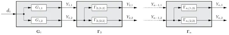
The structure of the cascaded system can be summarised in Figure 1 for a

perturbation d1 on the first vehicle. G1,1 and G1,2 are the elements of G1,

see equation (27). Yn is the Laplace transform ofyn. We writeYn,1 and Yn,2

the Laplace transforms of ∆yn and ˙yn, and Γn,1 and Γn,2 the SISO headway

to headway and speed to speed transfer functions. We have:

Yn,1 = Γn,1Yn−1,1, Yn,2 = Γn,2Yn−1,2, (38)

Finally, Γn,(1,2) and Γn,(2,2) are the terms of the second column in

equa-tion (37), and we have:

Figure 1: MIMO and SISO transfer functions of the studied cascaded system.

In the rest of the Section, we are interested in capturing the propagation of the headway and speed perturbations, which can be done by looking at either the MIMO transfer function or the SISO transfer functions.

a) Multiple Inputs Multiple Outputs (MIMO) system: the full MIMO

system is represented by transfer function Γn, see Figure 1. We calculate

the singular values of Γn(jω) to obtain its H∞ norm, following the

defini-tion of equadefini-tion (32). After some manipuladefini-tion, see Appendix A, sufficient conditions for strict string stability are:

fn,1 = 0, (40)

−2fn,2−1≥0. (41)

It can be seen that the sufficient conditions for strict string stability of the MIMO system are not useful in practice, as they are not compatible with the realistic driving constraints presented in equation (8).

b) Single Input Single Output (SISO) systems: given the conservativeness

of equations (40), (41), the strict string stability analysis of the SISO systems is critical. From equation (37-39) we immediately have the speed to speed transfer function:

Γn,2 =

sfn3+fn2

s2_+s(f

n,3−fn,1) +fn,2

. (42)

However, the propagation of the headway perturbations is not readily

obtain-able, and following equation (39), we need to express Yn−1,1 as a function of

Yn−1,2 to have an expression of Γn,1. As we remark thatYn−1,2−Yn,2 =sYn,1,

following equation (38), we have

Yn−1,2 =

sΓn,2

1−Γn,2

Yn−1,1, (43)

which reduces to

Yn−1,2 =

sfn,3+fn,2

s−fn,2

We therefore have the headway to headway transfer function:

Γn,1 =

sfn3+fn2

s2_+s(f

n,3−fn,1) +fn,2

, (45)

which is the same as the speed to speed transfer function, see equation (42).

The transfer functions Γn,k, withk ∈ {1,2}, have second order dynamics,

therefore we can get an analytical condition for L2 strict string stability. The

H∞ norm of Γn,k is the maximum gain |Γn,k(jω)| across all frequencies. We

have:

|Γn,k(jω)|=

s

ω2_f2

n,3+fn,22

(fn,2−ω2)2+ω2(fn,3 −fn,1)2

. (46)

Condition |Γn,k(jω)| ≤1 leads to equation

ω4 +ω2(f_n,2₁−2fn,3fn,1−2fn,2)≥0. (47)

That is, the L2 strict string stability condition is a simple condition on the

partial derivatives of the system: ∀ω∈_R+_,

|Γn,k(jω)| ≤1⇔fn,21−2fn,1fn,3−2fn,2 ≥0. (48)

Note that these conditions are the same conditions as the well-known string stability conditions derived for an infinite homogeneous traffic Wilson and Ward (2011). Note also that the discrepancy observed between the MIMO and SISO analysis may stem from the conservativeness of condition (34), and the fact that in the MIMO set-up the outputs are headway and speed and the input is just the speed of the previous vehicle.

5.3.2. L2 weak string stability

applying Definition 4, for a given l ∈ {i, ..., m} and n ∈ {l, ..., m}, a

sufficient condition for (l, n) weak string stability is:

n

Y

i=l+1 Γi

H∞

≤1. (49)

As an example, consider a system consisting of 3 vehicles, with a dis-turbance on vehicle 1. We work with the following partial derivative

val-ues: f21 = −0.075, f22 = 0.091, f23 = 0.55, and f31 = −0.26, f32 = 0.10,

Driver Model (IDM), a well-known physical model for reproducing realistic

traffic Kesting et al. (2010a). The L2 speed gains are ||Γ2,2||H∞ = 1.06,

||Γ3,2||H∞ = 1 and||Γ2,2Γ3,2||H∞ = 1, as we can observe in Figure 2. The

sys-tem is therefore (1,3) weakly string stable but not proved to be strict string stable. The automated vehicle (here vehicle 3) could compensate instabilities generated by the conventional vehicle (here vehicle 2). However, analytical conditions for achieving weak string stability are not easy to obtain as solving inequality (49) requires solving an 8 degree polynomial equation.

Figure 2: System of 3 vehicles: Bode plots of|Γ2,2(jω)|,|Γ3,2(jω)|and|Γ2,2(jω)Γ3,2(jω)|.

Remark 5. Note that, ∀k ∈ {1,2},

Qn

i=l+1Γi,k

_H∞ ≤1 is equivalent to

Qn

i=l+1Γi,k

H∞ = 1, as ∀i∈ {1, .., m}, we have |Γi,k(0)|= 1.

5.3.3. L∞ strict string stability

as discussed in Section 4, L∞ string stability is more practical than L2

of the early works to introduce the L∞-induced norm of a linear map, that

is the L1 norm of its impulse response, are the ones of Vidyasagar (1986);

Dahleh and Pearson (1987). This means that the condition to guaranteeL∞

strict string stability is to have the L1 norm of the impulse response less

than 1. It is known from Boyd and Barratt (????) that the H∞ norm is

upper bounded by the L∞-induced norm, and that for non-negative impulse

responses, those norms are identical. Therefore, if we look at the transfer functions of equations (42), (45), necessary and sufficient conditions for hav-ing a monotonic step response are non-imaginary poles and negative zeros, which leads to:

(fn,3 −fn,1)2−4fn,2 ≥0, (50)

−fn,2 fn,3

<0. (51)

Note that the conditions (51) is always verified due to the physical rela-tion (8). It is interesting to investigate which equarela-tion is the most conser-vative between (48) and (50). In fact, by substracting equation (48) from

equation (50), we can verify that theL2 strict stability condition is stronger

than the condition for the equality of the norms if f_n,2₃ ≥2fn,2, which we

ex-pect to be almost always verified for realistic parameter values. In summary, we have:

f_n,2₃ ≥2fn,2 ⇒(L∞ stability =L2 stability), (52)

and if condition (52) is not verified we only haveL∞stability⇒ L2 stability.

To our knowledge, whereas equation (48) is well-known to the traffic flow theory community, equations (45), (50) and (52) are novel conditions for the investigated car-following dynamics of equations (2) and (3).

5.4. Closed vehicle systems

We conclude the Section on stability results with the particular case of

closed systems. Closed vehicle systems, where vehicle 1 follows vehicle m,

By analogy with equation (21), the system matrix ac ∈ R2(m+1)×2(m+1) for a closed system can be written as

ac=        

a1,1 0 . . . 0 a1,0

a2,0 . .. ... ... 0

0 . .. ... ... ...

..

. . .. ... ... 0

0 . . . 0 am,0 am,1

        . (53)

For disturbance inputdi at vehiclei, wherei >2, we no longer haveyn(t) = 0

for n < i since now the vehicles n < i are affected by the disturbance on

vehicle i. The dynamics of vehicle i are now written as

Yi(s) = Γi(s)Yi−1(s) + (sI−ai,1)−1Di(s). (54)

In the case where the disturbance d1 in on vehicle 1, we have Y1(s) =

Γ1(s)Ym(s) + (sI−a1,1)−1D1(s), where Γ1(s) is the transfer function for

vehicle m to vehicle 1. We then have

Yi(s) = m

Y

j=1

Γj(s)Yj(s) + (sI−ai,1)−1Di(s), (55)

and finally, with di, ∀i ∈ {1, ..., m}, being the only non-zero component, we

have

Yi(s) = I− m

Y

j=1 Γj(s)

!−1

Gi(s)Di(s). (56)

5.4.1. SISO homogeneous case

we investigate the particular case where di ∈ R, i ≥ 1, yn ∈ R, ∀n ∈

{1, . . . , m}, ∀k ∈ {1,2}, Γn,k = Γ1. Following Remark 1 and equation (56),

as (an,1) is a Hurwitz matrix, exponential stability is achieved when the poles

of (1−Γn

1)

−1 _{have negative real parts. We factorise (1−Γ}n

1) as

1−Γn₁ = (1−Γ1)

m−1

Y

k=1

Γ1−e

2ikπ m

, (57)

and developing from equation (42), the denominatorDcof (1−Γn1)−1 is equal

to

Dc= m−1

Y

k=0

s2−sf1+f3

e2ikπm −1

−f2

e2ikπm −1

Note that this expression closely resembles the condition for string stability in the infinite homogeneous case derived using the Fourier perturbation tech-nique Wilson and Ward (2011). The infinite homogeneous system is said to

be stable iff ∀k∈[0,2π], s2_{−s f}

1+f3 eik−1

−f2 eik−1

has negative

real parts. This condition can be shown to be equivalent to the L2 strict

stability condition of equation (48), see Monteil et al. (2014b).

5.4.2. General case

in the general case, exponential stability is achieved when the transfer function in equation (56) has poles with negative real parts. From equa-tion (37), we have

m

Y

j=1

Γj(s) =

1

Qm

j=1γj(s)

0 P1(s)

0 P2(s)

, (59)

where γi(s) =s2 +s(fj,3−fj,1) +fj,2, and P1(s) and P2(s) are polynomials

of degree m, with

P2(s) = m

Y

i=1

(fi2+sfi3). (60)

Given that∀i∈ {1, ..., m}, the solutions ofγi(s) = 0 have negative real parts,

the system is exponentially stable iff the solutions of the following equation

m

Y

i=1

γi(s)−P2(s) = 0, (61)

have negative real parts.

Remark 6. There are situations for which the closed vehicle system is

asymptotically stable but not strict string stable, i.e. equation (48) is not

verified. For example, for 3 homogeneous vehicles, choosing fn,1 = −0.075,

fn,2 = 0.091, fn,3 = 0.55 as in Section 5.3.2, with n ∈ {1, ...,3}, we have

||Γn||H∞ >1 while the eigenvalues of matrixac have negative real parts.

6. Simulation

6.1. Model selection and parameter distributions

The Intelligent Driver Model (IDM) Kesting et al. (2010b) defines

func-tion fn of equation (3) as:

fn( ˙xn,∆xn,∆ ˙xn) =a

"

1−

˙ xn Vmax,n

4

−

s?_{( ˙x}

n,∆ ˙xn)

∆xn−ln

2#

, (62)

where

s?( ˙xn,∆ ˙xn) =s0,n+ max

0,x˙nTn− ˙ xn∆ ˙xn 2√anbn

, (63)

where the following behavioural parameters are specific to vehiclen: Vmax,nis

the desired free-flow speed, Tn is the safe time headway, an is the maximum

tolerated acceleration, bn is the comfortable deceleration, and s0,n is the

minimum stopping distance.

In order to reproduce realistic heterogeneous traffic in simulation, we have developed a complete methodology to perform robust offline parameter iden-tification starting from noisy trajectory data Monteil and Bouroche (????), which involves sensitivity analysis, point estimation and interval estimation. The parameter estimates we use here are the outputs of this methodology, for the 3 most left lanes of the well-known US101 NGSIM dataset IEEE (2005), during morning peak time (7:50am to 8:05am). The estimates were

found to fit log-normal distributions for parameters a and b and normal

distributions for parameters T and s0. The mean and standard deviations

are ma = 0.77 m s−2, σa = 0.42 m s−2, mb = 1.1 m s−2, σb = 0.43 m s−2,

mT = 1.5 s,σT = 0.57 s,ms0 = 2 m, andσs0 = 0.5 m. To reproduce

heteroge-nous traffic, the parameters are sampled from these distributions truncated

at the physical bounds chosen as in the literature: a ∈ [0.3,3], b ∈ [0.3,3],

T ∈ [0.3,3], s0 ∈ [0.5,3.5] Punzo et al. (2015). With Vmax = 33 m s−1

roughly corresponding to the speed limit of the section, see Punzo et al.

(2015), and taking for instance an equilibrium speed of Veq = Vmax/2, this

gives for an average vehiclen f_n,2₁−2fn,1fn,3−2fn,2 =−0.063, meaning that

parameters are distributed so that the L2 string stability condition is not

verified for a number of vehicles. In the remainder of the paper we write Sn :=fn21−2fn,1fn,3−2fn,2.

6.2. Homogeneous traffic: L2 strict string stability

6.2.1. Relevance of the strict string stability condition

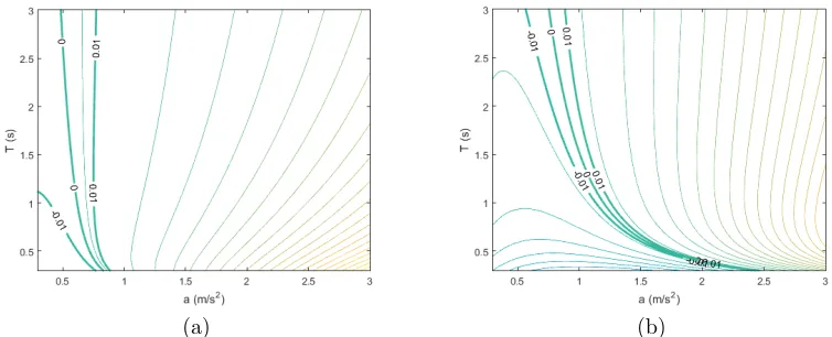
since the automated vehicles obey the IDM car-following model, it is of interest to investigate the parameter space for which the model exhibits strict and weak string stable behaviour. In this subsection we focus on the evolution

of the two most sensitive parameters, parameters a and T, see Punzo et al.

(2015), to gain insights on the possibilities to reach string stable behaviour with realistic parameters values. The rest of the parameters are chosen to

have realistic values, see Section 6.1, i.e. b = 1.1 m s−2, s0 = 2 m and

Vmax= 33 m s−1.

(a) (b)

Figure 3: Contour lines of the string stability coefficient Sn for (a) Veq = 2Vmax/3, (b) Veq=Vmax/3.

Figure 3 plots the contour lines of the string stability coefficient Sn. It

can be seen that the limit between string stability and string instability

de-pends on the traffic equilibrium speed. For low equilibrium speeds ofVmax/3,

which roughly corresponds to the value observed for the NGSIM data set,

we approximately need a ≥1.1 m s−2 with T ≥1.6 s to have a string stable

system (positiveSn). The instability domain is increased as we move towards

lower equilibrium speeds.

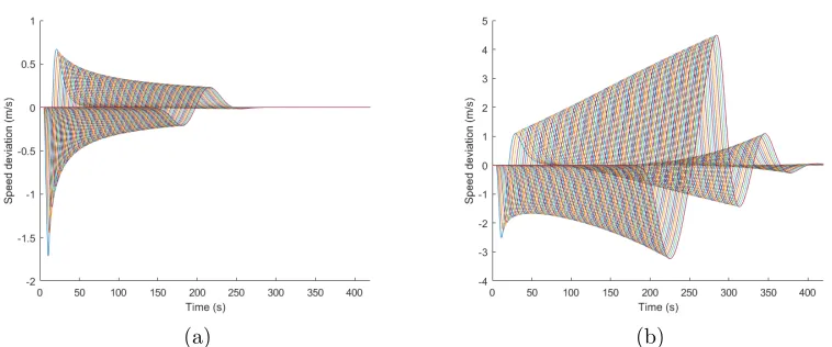
6.2.2. Strictly string stable vs strictly string unstable traffic

for the previously defined parameters, with T = 1.5 s, Veq = Vmax/2,

consider a string unstable system witha = 0.47 m s−2, and soSn =−0.018<

0; and a string stable system fora= 0.87 m s−2, and soSn >0. A disturbance

t1 = 5 s andt2 = 10 s. Note that this actually corresponds to the sum of two

opposed input steps, one happening at t1 = 5 s and one at t2 = 10 s.

(a) (b)

Figure 4: Evolution of the speed perturbations under a disturbance of A=−1 m s−2 _as function of the vehicle number for string stable and string unstable systems: (a)L2norm; (b)L∞ norm.

(a) (b)

Figure 5: Evolution of the speed perturbation following a disturbance of A=−1 m s−2 for (a) a strictly string stable system, (b) a strictly string unstable system.

The L2 norms of the speed perturbations are computed using an Euler

sum over the simulation time steps. It can be seen from Figure 4 that, in

with the vehicle number. Conversely, in the strictly string unstable case, it

can be seen that while the L∞ norm initially decreases, both norms tend to

increase after a certain vehicle number is reached. This is in accordance with the conclusions of Section 5.3. Figure 5 displays the evolution of the speed perturbation for all the vehicles in both strictly string stable and strictly string unstable cases. The string stability property means that the pertur-bation fades away. Note that we could have focused on the evolution of the headway perturbation equivalently as it leads to similar observations, as per equations (42), (45).

A last remark is made in the light of Figures 4 and 5. It is observed that the perturbation does not completely vanish, i.e. the bounded disturbance

is not attenuated to a perfect zero L2 norm as we move downstream. This is

related to the fact that||Γn,2||H∞ asymptotically converges towards Γn,2(0) =

1, see equation (48) and Figure 2, and that (34) is not a strict inequality, which means that the strict string stability condition does not require long-wave perturbations to be attenuated at a specific rate. Therefore, a stronger

condition than L2 strict string stability would be to force a sharper decrease

of the Bode plot for low frequencies, see Figure 2.

6.2.3. Nonlinear vs linear string stability: empirical observations

let us now briefly discuss the dependence of string stability on the size

of the disturbance. For the situation where a = 1.55 m s−2, and T = 0.8 s,

b = 1.7 m s−2, we have Sn = 0.0038>0. Figure 6a presents the evolution of

the time-position diagram for a disturbance of −7 m s−2 _{between t}

1 and t2

and Figure 6b presents the evolution of theL2norm of the speed perturbation

for varying disturbances.

It can be seen that, for disturbances of−5 m s−2 _{and−7 m s}−2_{, the values}

of theL2norm of the speed perturbation are growing as we move downstream

the vehicle system. This contradicts the string stability condition (48). We

see that, for a disturbance of −7 m s−2_{, the perturbation is being amplified}

until the vehicles completely stop, and the L2 norm seems to be unbounded.

For other disturbances, Figure 6b shows that the slope of the L2 norm curve

seems to be decreasing as we move downstream the vehicle system. Finally,

when the intensity of the disturbance is kept within realistic values, i.e. A <

−5 m s−2_{, theL}

2 norms appear to remain bounded as the number of vehicles

in the system is increased.

(a) (b)

Figure 6: Evolution of the (a) time vs position diagram for a string stable system following a disturbance ofA=−7 m s−2_{; (b)L}

2 norm of the speed perturbation for a string stable system and varying accelerations inputs.

time-space, the linearised dynamics which satisfy the string stability condi-tion is not valid anymore, and another linearisacondi-tion about a lower equilib-rium speed would indicate string instability, as Figure 3 suggests. Besides, the car-following formulation we consider does not deal with the zero speed constraint, i.e. the fact that vehicles cannot have negative speeds.

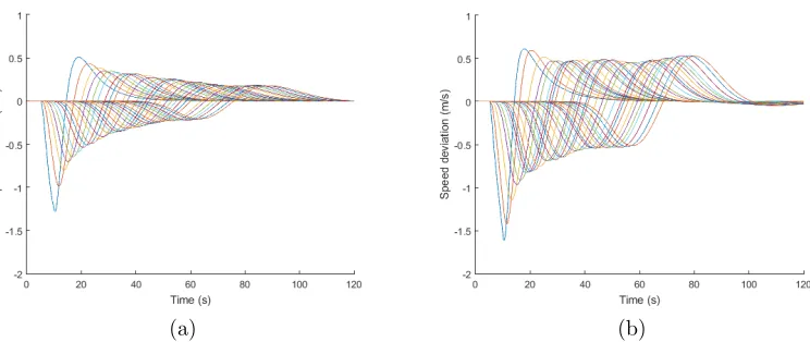
6.3. Heterogeneous traffic: L2 weak strict string stability

In this section we present an example that highlights the relevance of verifying the weak string stability condition, see equation (49). We consider a system composed of 30 vehicles having different behaviour, and we introduce

a disturbance of −1 m s−2 _{on vehicle 1 between t}

1 and t2. The variability

in the vehicle system is introduced by sampling parameters a and T from

truncated distributions as described in Section 6.1. For instance, we can

get a (0,30) weakly string stable system, i.e. Q30

i=1||Γi,2||H∞ ≤ 1, when

a and T are sampled from the distributions presented in Section 6.1 but

defining a ∈ [0.5,3] and T ∈ [1.1,3]; and we can get a (0,30) weakly string

unstable system, i.e. Q30

i=1||Γi,2||H∞ = 1.94 > 1, by defining a ∈ [0.3,1]

and T ∈ [0.3,2]. Note that the (0,30) weakly string stable and weakly

string unstable systems are obtained for particular samples of the truncated distributions.

(a) (b)

Figure 7: Evolution of the speed perturbation for successive vehicles in the case of: (a) (0,30) weak string stability; (b) (0,30) weak string instability.

system. It appears that the speed deviation is being damped in the weakly string stable case, despite the presence of 8 strictly string unstable vehicles in the considered vehicle system, and is being amplified in the weakly string unstable case, despite the presence of 9 strictly string stable vehicles.

In the remainder of this paper, we will investigate how to tune the be-havioural parameters of the automated vehicles so as to increase the weak string stability of the traffic flow.

7. Parameter optimisation

In this section, the automated vehicles update their longitudinal dynam-ics according to the IDM car-following model. We formulate the following optimisation problem: the vehicle behavioural parameters of each automated vehicle are picked to maximise the strict/weak string stability of the system, while minimising the distance between their parameter values and the vehicle behavioural parameters when there is no control, e.g. in the case of a par-tially automated vehicle with automated and non-automated driving modes, when the automated mode is deactivated. Note that we have made available a simple example of the code at this hyperlink.

Remark 7. Note that we make the choice to rely on in-vehicle sensors

Another way of increasing string stability is to utilise the car-following model structure itself to integrate V2V communication, see Monteil et al. (2014b); Ngoduy (2015) for instance, however by doing that the safe structure of car-following dynamics is lost, i.e. collisions may occur. Our approach of op-timising the car-following parameters is key to preserving the safe structure of the car-following dynamics. This enables the design of safe ACC systems that takes into consideration the driving behaviour of the surrounding vehi-cles in heterogeneous traffic as well as the driving comfort of the driver in the automated vehicle.

7.1. Generic formulation of the optimisation problem

LetT denote the joint distribution of the car-following parameters. The

vector of parameters θi ∈ Rl, i ∈ {1, ..., m}, defining the dynamics of each

vehicleiis sampled from this distribution. We write the covariance matrix of

T asΣT ∈Rk×k(R). When there is no correlation between parameters, as in

Section 6.1, ΣT is diagonal, and the elements of the diagonal are the inverses

of the standard deviations of each parameter. For each automated vehicle

indexed n, we seek to optimise thek ∈ {1, ..., l}parametersθn, with Θ ⊂Rk

denoting the admissible set of parameter values, e.g. the physical bounds of

the parameters defined in section 6.1. Therefore we have θn ∈ Θ. In the

case of a partially-automated vehicle, ˆθn denotes the estimated behavioural

parameters for vehicle n when the automated mode is deactivated; in the

case of a fully-automated vehicle, ˆθn designates average comfortable driving

parameters.

7.1.1. Relaxation of weak string stability

in Section 5.3.2, we discussed how automated vehicles can be used to achieve weak string stability. However, there exist situations for which this is not possible: for example, consider a system of 3 vehicles with parameters

a1 = 0.58 m s−2, a2 = 0.35 m s−2, a3 = 0.39 m s−2, and T1 = 1.76 s, T2 =

1.26 s,T3 = 1.43 s. The rest of the parameters are chosen asVmax= 33 m s−1,

b = 1.1 m s−2, and s0 = 2 m as in Section 6.1, and Veq = Vmax/3. For this

situation, we haveQ3

i=1||Γi,2||H∞ = 1.12>1, and after numerical simulations

we find no values of a4 ∈[0.3,3] andT4 ∈[0.3,3] leading to

Q4

i=1||Γi,2||H∞ = 1. This means that the weak string stability constraint of equation (49) can not be used as a hard constraint to an optimisation policy. Consequently, in

the next sections we relax constraint Q4

i=1||Γi,2||H∞ = 1 to Q4_i=1||Γi,2||H∞ <

7.1.2. Optimisation problem

let i and j be the farthest upstream and downstream vehicles for which

parameter estimates ˆθi and ˆθj are known. We have 1 ≤ i ≤ n ≤ j ≤

m. If there is no knowledge of the behaviour of upstream and downstream

vehicles, then i = j = n. Constraints are placed on the L2 gain between

the speed perturbation of vehiclei−1 and the speed perturbation of vehicle

j, i.e reflecting our aim of achieving (i −1, j) weak string instability, see

equation (49). The decision variables are the behavioural parameters θn of

the partially-automated vehicle n.

We propose the following optimisation problem to capture these design requirements:

min θn,γ

αγ + 1

k

θn−θˆn

Σ−1_T θn−θˆn

T

, (64)

s.t.







θn ∈Θ, ∀(i, j)∈ Nn,

||Γi,2· · ·Γj,2||H∞ ≤γ

(65)

where the objective is to minimise the distance between the optimised

param-eters θn and the vector of parameters of the vehicle ˆθn when the automation

mode is deactivated, as well as to minimise γ. Constant α ∈ _R∗

+ is a

de-sign parameter. Nn designates the set of pairs of neighbouring upstream

and downstream vehicles for which parameter estimates (ˆθi)i∈Nn are known,

with i ≤ n ≤ j. The (i−1, j) weak string stability condition is relaxed as

discussed in Section 7.1.1.

Remark 8. Note that the minimisation of the H∞ norm of the

input-output transfer function ||Gi,2Γi+1,2· · ·Γj,2||H∞ could be formulated as

an-other constraint.

Remark 9. Regarding the values ofiandj, in practice, automated vehicles

are equipped with sensors which can enable parameter estimation for only a few leading/following vehicles. Looking at equation (3), the acceleration and

speed of vehiclen, and the relative positions and speeds between vehiclenand

vehiclen−1 need to be tracked to be able to estimateθnvia static parameter

estimation techniques, see e.g. Monteil et al. (2015). Considering that only the positions and speeds of 2 upstream and downstream vehicles can be

tracked with in-vehicle sensors, we rarely havei < n−1 andj > n+ 2 unless

7.1.3. Limitations of weak string stability

when the knowledge of behavioural parameters is limited to only a few

leaders and followers, there exist situations for which the (i−1, j) weak string

stability constraint is verified but the (i−1−i1, j+j1) weak string stability

constraint is not, for giveni1, j1 ∈N. For example, takingi=j =n, we have

||Γn,2||H∞ = 1 and ||Γn,2Γn−1,2||H∞ > 1 for the following parameter values:

an = 0.9 m s−2,bn = 0.9 m s−2,Tn = 2.5 s,an−1 = 0.5 m s−2,bn−1 = 1.7 m s−2,

Tn−1 = 0.8 s, withVmax = 33 m s−1,s0 = 2 m, andVeq =Vmax/3. This means

that the verification of the (i−1, j) weak string stability is not sufficient to

ensure a (0, m) weakly string stable system. However, there exist two ways

to address this issue in order to provide a more stable system dynamics. The

first one consists in considering the minimisation of the input-output L2 gain

as well, that is the minimisation of kGn,2kH∞. The second one consists in

adding one (or various) fictitious unstable leading or following vehicle(s), i.e worst case vehicle(s), which will eventually lead to more extreme parameter values compensating the fictitious instabilities. For instance, let us consider

the case where the parameters of only vehiclen and vehiclen−1 are known.

Then, introducing a worst case vehicle with parametersθwc, we now perform

the minimisation of ||Γwc,2Γn,2Γn−1,2||H∞.

7.2. LMI formulation of the optimisation problem

We can rewrite constraints (65) as Linear Matrix Inequalities Boyd et al. (1994). Starting from equation (10) and combining the linearised dynamics

of cars i,...,j, with i, j ∈ Nn and i ≤ j, we write the following linearised

system dynamics:

˙

yi,j =Ai,jyi,j +bi,jui,j, (66) hi,j =ci,jyi,j (67)

whereyT

i,j = [yiT,yTi+1,· · · ,yTj],uTi,j = [uTi ,uTi+1,· · · ,uTj],bi,j ∈R2(j−i+1)×2(j−i+1)

andci,j ∈R2(j−i+1)×2(j−i+1)are the input weighting and observation matrices,

and

Ai,j =

       

ai,1 0 . . . 0

ai+1,0 . .. ... ... ...

0 . .. ... ... ...

..

. . .. ... ... 0

0 . . . 0 aj,0 aj,1

As the speed ˙yj is observed, we have

ci,j =

       

0 . . . 0

..

. . .. ... ... ...

..

. . .. ... ... ...

..

. . .. ... 0 0

0 . . . 0 1

        . (69)

The stability constraint is on the L2 gain between speed perturbation ˙yi−1

and speed perturbation ˙yj. We consider the input as yi−1. Following

equa-tion (10), since the first column of matrix ai,0 consists of zeros, only ˙yi−1

acts as input to the yj dynamics, i.e. the ∆yi−1 term has no effect since it

is multiplied by the zeros in the first column of ai,0, which makes it a SISO

system. We can therefore write

bi,j,1 =

       

0 1 0 . . . 0

..

. fi,3 0 . .. ...

..

. . .. 0 ... ...

..

. . .. ... ... ...

0 . . . 0

        . (70)

Therefore, using the LMI characterisation of the L2 gain, see Boyd et al.

(1994); Isidori (2011), we can reformulate the optimisation problem (64), (65) as:

min θn,Xi,j,γ

αγ+ 1

k

θn−θˆn

ΣT−1

θn−θˆn

(71) s.t.               

θn ∈Θ, ∀(i, j)∈ Nn,





AT

i,jXi,j+Xi,jAi,j Xi,jbi,j,1 cTi,j bT

i,j,1Xi,j −γIi,j 0

ci,j 0 −γIi,j



≺0,

Xi,j 0,

(72)

where the matrices Ai,j depend on θn, see equations (12), (13), (68), Xi,j ∈

R2(j−i+1)×2(j−i+1), and Ii,j ∈ R2(j−i+1)×2(j−i+1) is the identity matrix. This

car-following model θn, and not jointly convex in Aij and Xij. Even

af-ter linearising or convexifying the car-following model, assuming ΣT−1 to

be positive semi-definite, we would still be facing a biconvex optimisation problem. In this paper, we explore the car-following model parameter space using simulated annealing and solve the convex part of the optimisation using

cvx Grant and Boyd (2015) to obtain Xi,j andγ at each iteration. Note that

other heuristics such as the Alternate Convex Search (ACS) Gorski et al. (2007) may be of use.

Remark 10. The constraint concerning the minimisation of the L2 gain

between the disturbance di and the speed perturbation ˙yj, mentioned in

Remark 8, can also be formulated as LMI.

7.3. Simulation analyses and main results

7.3.1. Scenario and stochastic variables

although we performed numerous simulation experiments, in this section, we only show the results obtained for a representative example. We consider

a system of 30 vehicles, i.e. m = 30, and vehicle n = 0 evolving at an

equilibrium speed Veq = Vmax/3, as roughly observed in the NGSIM data

set, see section 6.2.1. Vehicle car-following parameters are sampled from the

joint distribution T, as defined in section 6.1. We introduce an acceleration

perturbation to vehicle 1, which is forced to be a non-automated vehicle. This perturbation takes the form of a PRBS input sequence of amplitude

[−1,+1], which remains constant over time intervals ranging from 2 s to 5 s

and has a duration of 1 min. The simulation length is set to 4 min as, given the considered perturbation, this is the time needed to cover all of the effects of perturbation propagation on the 30 vehicle trajectories. The stochastic variables are the sampled parameters of the 30 vehicles, the acceleration PRBS inputs, the position of the automated vehicles in the vehicle system,

and the number of automated vehicles in the vehicle system. Then, we

perform 25×4 simulations: we repeat the simulation 25 times to consider

7.3.2. Evolution of theL2 norm of the speed perturbation and distribution of

optimised parameters

we focus on tuning parameters a, b, and T for the automated vehicles

according to optimisation (72), i.e. the tolerated acceleration, comfortable

deceleration and safe time headway parameters. We choose α = 103_{, and}

work with i=n−1 and j =n+ 2, see Section 7.1.2.

Figure 8: Evolution of the L2 norm of the speed perturbation in the vehicle system for growing proportions of automated vehicles: 0%, 10%, 20%, 30%.

First, Figure 8 displays the influence of the optimisation strategy (72) on

the evolution of the L2 norm of the speed perturbation in the system,

fol-lowing the introduced PRBS acceleration inputs, for different proportion of

automated vehicles. We plot the average values and errors bars of ±1

stan-dard deviation over the 25 simulations. The error bars show the impact of the stochastic variables over the outcome of the minimisation. The positive effects are clearly visible: an increasing percentage of automated vehicles

of the speed perturbation. Here the (0,30) weak string stability condition,

i.e. decrease of the L2 norm of the speed perturbation, is verified when 30%

vehicles are automated, which makes sense as the (n−2, n+ 2) weak string

stability condition of (72) involves a total of 4 vehicles, which means that

an average of 1/4 = 25% of automated vehicles should be enough to

guar-antee (0,30) weak string stability provided the automated vehicles are well

dispersed. Note that the PRBS input considered is actually a linear

combi-nation of step inputs of ±2 m s−2_{, which are strong deceleration/acceleration}

inputs in realistic traffic. Note also that it was observed in section 6.2.3 and Figure 6 that for such inputs the verification of the strict string stability for

homogeneous traffic still leads to a decrease of the L2 norm of the speed

perturbation.

Figure 9: Evolution of the relativeL2norm of the speed perturbation in the vehicle system for different proportions of automated vehicles: 10%, 20%, 30%.

minimum and maximum values of the deviation from the value of the L2 norm of the speed perturbation without any automated vehicles, for 3, 6 and 9 automated vehicles, i.e. proportions of 10%, 20% and 30%. We observe that the automated vehicles with parameters derived from the optimisation

strategy (72) contribute to systematically decrease the value of the L2 norm

of the speed perturbation, i.e. negative relative L2 norms. In that sense, the

proposed optimisation algorithm (72) consistently increases the traffic flow stability of the heterogeneous system.

Figure 10: Standard vs optimised distributions of automated vehicle parametera.

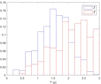
Finally, we look at the distributions of the optimised parameters ˜a, ˜T and

˜

b, displayed in Figures 10, 11, 12. As might be expected, the distributions

are shifted but are still realistic, i.e. lead to reasonable driving behaviour by the automated vehicles. We observe that the optimisation strategy (72)

pushes parameters a and T towards higher values and parameter b towards

Figure 11: Standard vs optimised distributions of automated vehicle parameterT.

safe time headway T gives more time for vehicles to damp perturbations;

a higher tolerated acceleration helps recover the equilibrium speed faster; a smaller comfortable deceleration results in less sharp braking and helps to smooth perturbations.

We can also observe that parameters b and T are sometimes pushed

to-wards the limits of the selected physical bounds, i.e. in this case T = 3s

and b = 0.3m s2_{. When this is the case, one idea to provide more flexibility}

to guarantee weak string stability, see Section 7.1.1, is to increase the upper

bound Tup of the safe time headway parameter T, which is not a critical

Figure 12: Standard vs optimised distributions of automated vehicle parameter b.

7.3.3. Systematically enforcing more stable dynamics with very few auto-mated vehicles

with very few automated vehicles in the vehicle system, and when the parameters of only a few leading and following vehicles are known, we might be interested in investigating how to enforce an even more stable dynamics. To do so we can introduce fictitious unstable vehicles, see section 7.1.3.

We consider i = n−1 and j = n−2, and 3 automated vehicles in the

system, i.e. NbAut = 3. A fictitious worst case unstable vehicle n−2 is

introduced with parameters an−2 = 0.3 m s−2, Tn−2 = 0.3 s, bn−2 = 3 m s−2.

Figure 13 shows the results of the optimisation without and with the ficti-tious introduced vehicle, for 2 different admissible upper values of parameter

Tup, Tup = 3 s and Tup = 5 s. It is visible that adding one fictitious unstable

Figure 13: Evolution of theL2norm of the speed perturbation in the vehicle system with no automated vehicle; 3 automated vehicles and no fictitious vehicle; 3 automated vehicles, 1 fictitious vehicle and Tup= 3 s; 3 automated vehicles, 1 fictitious vehicle andTup= 5 s.

the admissible set of parameter values Θ. By increasing the upper bound of

the admissible safe time headway Tn, we are able to bypass this limitation

and reach (0,30) weak string stability with only 3 automated vehicles in the

vehicle system. This strategy may lead to less realistic and less comfortable driving behaviour, as parameters tend to move towards their upper/lower admissible bounds. However the physical bounds can be selected

appropri-ately, as for instance parameter T is less critical than parameters a and b in

terms of vehicle capabilities and driving comfort, although increasing T may

encourage vehicles to change lanes and enter the empty slots created. Finally, the overall conclusion is that the number of automated vehicles needed to prevent perturbation growth can be reduced depending on the following parameters of the optimisation strategy: the number of vehicles for

set of admissible parameters Θ, and the parameters of introduced fictitious unstable vehicles. Given a string of vehicles, a small number of automated vehicles is enough to damp the effect of realistic perturbations that would otherwise grow.

8. Conclusion

This paper appliesL2 linear control theory to linearised systems of

vehi-cles moving according to realistic car-following models. The contributions are the following: a general framework for investigating the stability and string stability of heterogeneous traffic in the frequency domain is introduced (most previous studies assume homogeneous traffic); the definition of weak stabil-ity is introduced and its relevance in a traffic environment with a mix of automated and non-automated vehicles is highlighted; conditions for input-output stability and string stability are given for heterogeneous traffic, and

for single and multiple outputs; the relation between L2 and L∞ string

sta-bility is presented; the equivalence between string stasta-bility and asymptotic stability is showed not to hold for closed loop systems; simulations under-line the critical feature of nonunder-linearities; an optimisation strategy to tune the behavioural parameters is proposed as well as its LMI formulation; the optimisation is applied to realistic data yielding promising results: a small proportion of automated vehicles, that behave similarly to their drivers, can greatly and systematically contribute to increasing traffic flow stability.

With regard to future work, (i) the impact of the non-linear dynamics, and (ii) the reasons for perturbation growth and boundedness under high acceleration inputs as the number of vehicles increases remain open questions. Regarding optimisation, (iii) the formulated LMI optimisation problem may be solved more efficiently. Finally, regarding control, (iv) the mapping of this work with online parameter identification of drivers’ behavioural parameters, and the consideration of parameters uncertainty for the design of control strategies remain to be studied.

Appendix A.

Singular valuesσmax are defined as follows. For any F∈R2×2,

σmax(F(jω)) =

p

where F(jω)∗ is the conjugate transpose of F(jω) and λmax(F(jω)∗F(jω))

denotes the maximum of the nonzero eigenvalues of F(jω)∗F(jω).

Following equation (37), the productΓ∗_n(jω)Γn(jω) is written:

Γ∗_nΓn = 1

D∗

nDn

0 0

0 ω2_{(1 +f}2

n,3) +fn,21+fn,22

, (A.1)

where D∗_nDn is equal to:

D_n∗Dn =ω4+ω2 (fn,3−fn,1)2−2fn,2

+f_n,2₂. (A.2)

The two eigenvalues λ1 and λ2 of Γn∗(jω)Γn(jω) immediately follow:

λ1(ω) = 0, (A.3)

λ2(ω) =

ω2_{(1 +f}2

n,3) +fn,22+fn,21

ω4_+ω2_((f

n,3−fn,1)2−2fn,2) +fn,22

. (A.4)

which gives

σmax(Γn(jω)) =

p

λ2(ω). (A.5)

We recall that, by definition, see equation (32), we have

||Γn||H∞ = sup

ω∈R

σmax(Γn(jω)).

The sufficient condition for strict string stability is written ||Γn||H∞ ≤1, see

equation (36), which is equivalent to λ2(ω)≤1.

Developing λ2(ω) ≤ 1, and writing Ω = ω2, we obtain a polynomial of

order 2 in Ω:

Ω2+ Ω(f_n,2₁−2fn,1fn,3−2fn,2−1)−fn,21 ≥0. (A.6)

As this inequality must be verified ∀Ω∈_R+, we must have fn,1 = 0, and the

following sufficient conditions follow:

fn,1 = 0, (A.7)

Acknowledgment

This work was supported by SFI grants 11/PI/1177, 13/RC/2077 and 10/IN.1/I2980.

Bando, M., Hasebe, K., Nakayama, A., Shibata, A., Sugiyama, Y., 1995. Dynamical model of traffic congestion and numerical simulation. Phys. Rev. E 51 (2), 1035–1042.

Boyd, S., El Ghaoui, L., Feron, E., Balakrishnan, V., Jun. 1994. Linear Matrix Inequalities in System and Control Theory. Vol. 15 of Studies in Applied Mathematics. SIAM, Philadelphia, PA.

Boyd, S. P., Barratt, C. H., ???? Linear controller design: limits of perfor-mance.

Dahleh, M., Pearson, J., 1987. lˆ{1}-optimal feedback controllers for mimo discrete-time systems. IEEE Transactions on Automatic Control 32 (4), 314–322.

Darbha, S., Rajagopal, K. R., 2005. Information flow and its relation to the stability of the motion of vehicles in a rigid formation. In: American Control Conference, 2005. Proceedings of the 2005. IEEE, pp. 1853–1858.

Desoer, C. A., Vidyasagar, M., 2009. Feedback Systems: Input-Output Prop-erties. R. E. OMalley, Ed. Philadelphia, PA, USA: SIAM.

di Bernardo, M., Salvi, A., Santini, S., Feb 2015. Distributed consensus strat-egy for platooning of vehicles in the presence of time-varying heterogeneous communication delays. IEEE Transactions on Intelligent Transportation Systems 16 (1), 102–112.

Frankel, J., Alvarez, L., Horowitz, R., Li, P., 1996. Safety oriented maneuvers for ivhs. Vehicle System Dynamics 26 (4), 271–299.

Gibson, T. E., Annaswamy, A. M., July 2015. Adaptive control and the definition of exponential stability. In: 2015 American Control Conference (ACC). pp. 1549–1554.

Grant, M., Boyd, S., 2015. Cvx: Matlab software for disciplined convex programming.

URL http://cvxr.com/cvx/

Hedrick, J. K., Tomizuka, M., Varaiya, P., 1994. Control issues in automated highway systems. IEEE Control Systems 14 (6), 21–32.

Hespanha, J., 2009. Linear Systems Theory. Princeton Press.

IEEE, 2005. Ngsim data sets.

URL http://ngsim-community.org/

Isidori, A., 2011. Robust stability via Hinfinity methods.

URL http://www.eeci-institute.eu/GSC2012/Photos-EECI/ EECI-GSC-2012-M9/Handout_1.pdf

Kesting, A., Treiber, M., Helbing, D., 2010a. Enhanced intelligent driver model to access the impact of driving strategies on traffic capacity. Philo-sophical Transactions of the Royal Society A 368, 4585–4605.

Kesting, A., Treiber, M., Helbing, D., 2010b. Enhanced intelligent driver model to access the impact of driving strategies on traffic capacity. Philo-sophical Transactions of the Royal Society of London A: Mathematical, Physical and Engineering Sciences 368 (1928), 4585–4605.

Klinge, S., Middleton, R. H., June 2009. String stability analysis of homoge-neous linear unidirectionally connected systems with nonzero initial con-ditions. In: Signals and Systems Conference (ISSC 2009), IET Irish. pp. 1–6.

Knorn, S., Donaire, A., Ag¨uero, J. C., Middleton, R. H., 2014.

Passivity-based control for multi-vehicle systems subject to string constraints. Au-tomatica 50 (12), 3224–3230.

Li, P., Alvarez, L., Horowitz, R., 1997. Ahs safe control laws for platoon leaders. IEEE Transactions on Control Systems Technology 5 (6), 614– 628.

Monteil, J., Billot, R., Sau, J., Buisson, C., El Faouzi, N.-E., 2014a. Calibra-tion, estimaCalibra-tion, and sampling issues of car-following parameters. Trans-portation Research Record: Journal of the TranTrans-portation Research Board, 131–140.

Monteil, J., Billot, R., Sau, J., El Faouzi, N.-E., 2014b. Linear and weakly nonlinear stability analyses of cooperative car-following models. IEEE Transactions on Intelligent Transportation Systems 15 (5), 1–13.

Monteil, J., Bouroche, M., ???? Robust parameter estimation of car-following parameters considering practical identifiability. ITSC 2016 conference.

Monteil, J., OHara, N., Cahill, V., Bouroche, M., 2015. Real-time estimation of drivers’ behaviour. In: Intelligent Transportation Systems (ITSC), 2015 IEEE 18th International Conference on. IEEE, pp. 2046–2052.

Monteil, J., Russo, G., July 2017. On the design of nonlinear distributed control protocols for platooning systems. IEEE Control Systems Letters 1 (1), 140–145.

Naus, G., Vugts, R., Ploeg, J., Van de Molengraft, M., Steinbuch, M., Nov 2010. String-stable CACC design and experimental validation: A frequency-domain approach. Vehicular Technology, IEEE Transactions on 59 (9), 4268–4279.

Newell, G., 2002. A simplified car-following theory: a lower order model. Transportation Research Part B: Methodological 36 (3), 195 – 205. URL http://www.sciencedirect.com/science/article/pii/ S0191261500000448

Ngoduy, D., 2015. Linear stability of a generalized multi-anticipative car following model with time delays. Communications in Nonlinear Science and Numerical Simulation 22 (13), 420 – 426.

URL http://www.sciencedirect.com/science/article/pii/ S100757041400402X