Sometimes Average is Best: The Importance of Averaging for Prediction using MCMC Inference in Topic Modeling

Sometimes Average is Best: The Importance of Averaging for Prediction

using

MCMC

Inference in Topic Modeling

Viet-An Nguyen

Computer Science

University of Maryland

College Park,

[email protected]

Jordan Boyd-Graber

Computer Science

University of Colorado

Boulder,

[email protected]

Philip Resnik

Linguistics and

University of Maryland

College Park,

[email protected]

Abstract

Markov chain Monte Carlo (MCMC)

approxi-mates the posterior distribution of latent vari-able models by generating many samples and averaging over them. In practice, however, it is often more convenient to cut corners, using only a single sample or following a suboptimal averaging strategy. We systematically study

dif-ferent strategies for averagingMCMCsamples

and show empirically that averaging properly leads to significant improvements in prediction.

1 Introduction

Probabilistic topic models are powerful methods to un-cover hidden thematic structures in text by projecting each document into a low dimensional space spanned by a set oftopics, each of which is a distribution over words. Topic models such as latent Dirichlet alloca-tion (Blei et al., 2003,LDA) and its extensions discover

these topics from text, which allows for effective ex-ploration, analysis, and summarization of the otherwise unstructured corpora (Blei, 2012; Blei, 2014).

In addition to exploratory data analysis, a typical goal of topic models is prediction. Given a set of

unanno-tated training data, unsupervised topic modelstry to

learn good topics that can generalize to unseen text.

Supervised topic modelsjointly capture both the text

and associatedmetadatasuch as a continuous response

variable (Blei and McAuliffe, 2007; Zhu et al., 2009; Nguyen et al., 2013), single label (Rosen-Zvi et al., 2004; Lacoste-Julien et al., 2008; Wang et al., 2009) or multiple labels (Ramage et al., 2009; Ramage et al., 2011) to predict metadata from text.

Probabilistic topic modeling requires estimating the posterior distribution. Exact computation of the poste-rior is often intractable, which motivates approximate inference techniques (Asuncion et al., 2009). One

popu-lar approach is Markov chain Monte Carlo (MCMC), a

class of inference algorithms to approximate the target

posterior distribution. To make prediction, MCMC

al-gorithms generate samples on training data to estimate corpus-level latent variables, and use them to generate samples to estimate document-level latent variables for test data. The underlying theory requires averaging on both training and test samples, but in practice it is often convenient to cut corners: either skip averaging entirely by using just the values of the last sample or use a single training sample and average over test samples.

We systematically study non-averaging and averaging

strategies when performing predictions usingMCMCin

topic modeling (Section 2). Using popular unsupervised (LDAin Section 3) and supervised (SLDAin Section 4)

topic models via thorough experimentation, we show empirically that cutting corners on averaging leads to consistently poorer prediction.

2 Learning and Predicting with MCMC

While reviewing all ofMCMCis beyond the scope of

this paper, we need to briefly review key concepts.1 _To

estimate a target density p(x)in a high-dimensional spaceX,MCMCgenerates samples{xt}Tt=1while

ex-ploringX using the Markov assumption. Under this

assumption, samplext+1depends on samplextonly,

forming aMarkov chain, which allows the sampler to

spend more time in the most important regions of the density. Two concepts control sample collection:

Burn-in B: Depending on the initial value of the

Markov chain, MCMC algorithms take time to reach

the target distribution. Thus, in practice, samples before a burn-in periodBare often discarded.

Sample-lagL: Averaging over samples to estimate the target distribution requires i.i.d. samples. However, future samples depend on the current samples (i.e., the Markov assumption). To avoid autocorrelation, we dis-card all but everyLsamples.

2.1 MCMC in Topic Modeling

As generative probabilistic models, topic models define a joint distribution over latent variables and observable evidence. In our setting, the latent variables consist of corpus-levelglobalvariablesgand document-level lo-calvariablesl; while the evidence consists of wordsw

and additional metadatay—the latter omitted in unsu-pervised models.

During training, MCMC estimates the posterior

p(g,lTR_|wTR_,yTR_{) by generating a training Markov} chainof TTR samples.2 Each training samplei pro-vides a set of fully realized global latent variablesgˆ(i), which can generate test data. During test time, given a 1_{For more details please refer to Neal (1993), Andrieu et}

al. (2003), Resnik and Hardisty (2010).

2_{We omit hyperparameters for clarity. We split data into}

training (TR) and testing (TE) folds, and denote the training iterationiand the testing iterationjwithin the corresponding Markov chains.

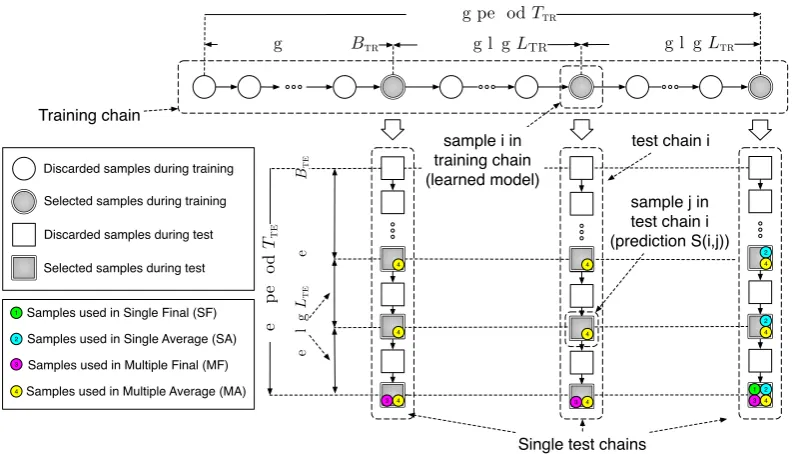
Training burn-inBtr Training lagLTR Training lagLtr Training periodTtr

Te

st

bu

rn

-in

Bte

Te

st

pe

ri

od

Tte

Te

st

lag

Lte

12 34 2 4 2 4

34 34

4 4

4 4

1

2

3

4

Samples used in Single Final (SF)

Samples used in Single Average (SA)

Samples used in Multiple Final (MF)

Samples used in Multiple Average (MA) Training chain

Single test chains sample i in

training chain (learned model)

test chain i

sample j in test chain i (prediction S(i,j)) Discarded samples during training

Discarded samples during test Selected samples during training

Selected samples during test

Figure 1: Illustration of training and test chains inMCMC, showing samples used in four prediction strategies studied

in this paper: Single Final (SF), Single Average (SA), Multiple Final (MF), and Multiple Average (MA).

learned model from training samplei, we generate atest Markov chainofTTEsamples to estimate the local latent variablesp(lTE_|wTE_{,gˆ(i))of test data. Each sample} jof test chainiprovides a fully estimated local latent variablesˆlTE_{(i, j)to make a prediction.}

Figure 1 shows an overview. To reduce the ef-fects of unconverged and autocorrelated samples,

dur-ing traindur-ing we use a burn-in period of BTR and a

sample-lag ofLTR iterations. We useTTR = {i|i ∈

(BTR, TTR]∧(i−BTR) mod LTR = 0}to denote the set of indices of the selected models. Similarly,BTE

and LTE are the test burn-in and sample-lag. The

set of indices of selected samples in test chains is

TTE={j|j∈(BTE, TTE]∧(j−BTE) modLTE= 0}.

2.2 Averaging Strategies

We useS(i, j)to denote the prediction obtained from samplejof the test chaini. We now discuss different strategies to obtain the final prediction:

• Single Final (SF)uses the last sample of last test

chain to obtain the predicted value,

SSF=S(TTR, TTE). (1) • Single Average (SA)averages over multiple

sam-ples in the last test chain

SSA= 1_|T TE|

X

j∈TTE

S(TTR, j). (2)

This is a common averaging strategy in which we obtain a point estimate of the global latent variables at the end of the training chain. Then, a single test chain is generated on the test data and multiple sam-ples of this test chain are averaged to obtain the final prediction (Chang, 2012; Singh et al., 2012; Jiang et al., 2012; Zhu et al., 2014).

• Multiple Final (MF)averages over the last

sam-ples of multiple test chains from multiple models

SMF= 1_|T TR|

X

i∈TTR

S(i, TTE). (3)

• Multiple Average (MA)averages over all samples

of multiple test chains for distinct models,

SMA= 1_|T TR|

1

|TTE| X

i∈TTR X

j∈TTE

S(i, j), (4)

3 Unsupervised Topic Models

We evaluate the predictive performance of the

unsu-pervised topic model LDA using different averaging

strategies in Section 2.

LDA: Proposed by Blei et al. in 2003,LDAposits that

each documentdis a multinomial distributionθdover

Ktopics, each of which is a multinomial distribution

φkover the vocabulary.LDA’s generative process is:

1. For each topick∈[1, K]

(a) Draw word distributionφk∼Dir(β)

2. For each documentd∈[1, D]

(a) Draw topic distributionθd ∼Dir(α)

(b) For each wordn∈[1, Nd]

i. Draw topiczd,n∼Mult(θd)

ii. Draw wordwd,n∼Mult(φzd,n)

InLDA, the global latent variables are topics{φk}Kk=1

and the local latent variables for each documentdare topic proportionsθd.

assigning tokennof training documentdto topickis p(zTR

d,n=k|z−TRd,n,w−TRd,n, wTRd,n=v)∝

N_TR−d,n_,d,k+α N_TR−d,n_,d,·+Kα·

N_TR−d,n_,k,v+β

N_TR−d,n_,k,·+V β, (5)

whereNTR,d,kis the number of tokens in the training

documentdassigned to topick, andNTR,k,vis the

num-ber of times word typevassigned to topick. Marginal

counts are denoted by ·, and−d,n _{denotes the count}

excluding the assignment of tokennin documentd. At each training iterationi, we estimate the distribu-tion over wordsφˆk(i)of topickas

ˆ

φk,v(i) =_NNTR,k,v(i) +β

TR,k,·(i) +V β (6)

where the countsNTR,k,v(i)andNTR,k,·(i)are taken at

training iterationi.

Test: Because we lack explicit topic annotations for these data (c.f. Nguyen et al. (2012)), we useperplexity– a widely-used metric to measure the predictive power of topic models on held-old documents. To compute

perplexity, we follow theestimatingθ method

(Wal-lach et al., 2009, Section 5.1) and evenly split each test

documentdintowTE1

d andwTEd2. We first run Gibbs

sampling onwTE1

d to estimate the topic proportionθˆdTE

of test documentd. The probability of assigning topick to tokenninwTE1

d isp(zd,nTE1=k|z−TEd,n1 ,wTE1,φˆ(i))∝

N_TE−d,n_1,d,k+α

N_TE−d,n_1,d,·+Kα·φˆk,wTEd,n1(i) (7)

whereNTE1,d,kis the number of tokens inwTEd1assigned

to topick. At each iterationjin test chaini, we can estimate the topic proportion vectorθˆTE

d (i, j)for test

documentdas

ˆ

θTE

d,k(i, j) = _NNTE1,d,k(i, j) +α

TE1,d,·(i, j) +Kα

(8)

where both the countsNTE1,d,k(i, j)andNTE1,d,·(i, j)

are taken using samplejof test chaini.

Prediction: Given θˆTE

d (i, j) and φˆ(i) at sample j

of test chain i, we compute the predicted

likeli-hood for each unseen token wTE2

d,n as S(i, j) ≡

p(wTE2

d,n|θˆdTE(i, j),φˆ(i)) =

P_K

k=1θˆd,kTE(i, j)·φˆk,wTE2

d,n(i).

Using different strategies described in Section 2, we obtain the final predicted likelihood for each un-seen token p(wTE2

d,n|θˆdTE,φˆ) and compute the

perplex-ity as exp−(P_dP_nlog(p(wTE2

d,n|θˆdTE,φˆ)))/NTE2

whereNTE2is the number of tokens inwTE2.

Setup: We use three Internet review datasets in our experiment. For all datasets, we preprocess by tokeniz-ing, removing stopwords, stemmtokeniz-ing, adding bigrams to

● ●

●

● _●

● ● ● ● ●

● ●

●

● _●

● ● ● ● ●

● ●

●

● _●

● ● ● ● ●

Restaurant Reviews

Movie Reviews

Hotel Reviews 1160

1200 1240

1950 2000 2050 2100 2150

750 775 800

600 700 800 900 1000

600 700 800 900 1000

600 700 800 900 1000

Number of training iterations

P

er

ple

xity

●

Multiple−Average Multiple−Final Single−Average Single−Final

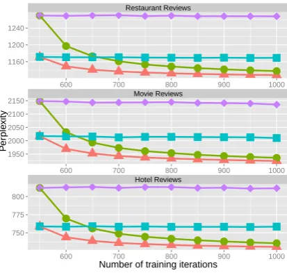
Figure 2: Perplexity ofLDAusing different averaging

strategies with different number of training iterations

TTR. Perplexity generally decreases with additional

training iterations, but the drop is more pronounced with multiple test chains.

the vocabulary, and we filter usingTF-IDFto obtain a

vocabulary of 10,000 words.3 _{The three datasets are:}

• HOTEL: 240,060 reviews of hotels from TripAdvi-sor (Wang et al., 2010).

• RESTAURANT: 25,459 reviews of restaurants from

Yelp (Jo and Oh, 2011).

• MOVIE: 5,006 reviews of movies from Rotten

Tomatoes (Pang and Lee, 2005)

We report cross-validated average performance over five folds, and useK = 50topics for all datasets. To update the hyperparameters, we use slice sampling (Wal-lach, 2008, p. 62).4

Results: Figure 2 shows the perplexity of the four averaging methods, computed with different number of training iterationsTTR.SAoutperformsSF, showing the benefits of averaging over multiple test samples from a single test chain. However, both multiple chain

methods (MFandMA) significantly outperform these

two methods.

This result is consistent with Asuncion et al. (2009), who run multiple training chains but a single test chain for each training chain and average over them. This is more costly since training chains are usually signif-icantly longer than test chains. In addition, multiple training chains are sensitive to their initialization.

3_{To find bigrams, we begin with bigram candidates that}

occur at least 10 times in the corpus and use aχ2_{test to filter} out those having aχ2_{value less than 5. We then treat selected} bigrams as single word types and add them to the vocabulary.

4_{MCMC setup: T}

TR = 1,000, BTR = 500, LTR = 50,

MSE

pR.squared 0.60

0.65 0.70 0.75

0.25 0.30 0.35 0.40

1000 2000 3000 4000 5000

1000 2000 3000 4000 5000

Number of iterations

(a) Restaurant reviews

MSE

pR.squared 9000

10000 11000 12000 13000

30000 31000 32000 33000 34000

1000 2000 3000 4000 5000

1000 2000 3000 4000 5000

Number of iterations

(b) Movie reviews

MSE

pR.squared 0.400

0.425 0.450 0.475 0.500

0.500 0.525 0.550 0.575 0.600

600 700 800 900 1000

600 700 800 900 1000

Number of iterations

(c) Hotel reviews

Multiple Average Multiple Final Single Average Single Final

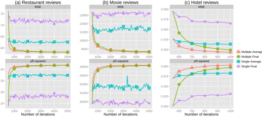
Figure 3: Performance ofSLDAusing different averaging strategies computed at each training iteration.

4 Supervised Topic Models

We evaluate the performance of different prediction methods using supervised latent Dirichlet allocation (SLDA) (Blei and McAuliffe, 2007) for sentiment

anal-ysis: predicting review ratings given review text. Each review text is the documentwdand the metadataydis

the associated rating.

SLDA: Going beyondLDA,SLDAcaptures the

rela-tionship between latent topics and metadata by mod-eling each document’s continuous response variable using a normal linear model, whose covariates are the document’s empirical distribution of topics:yd ∼

N(ηT_{z¯d, ρ)whereηis the regression parameter}

vec-tor andz¯d is the empirical distribution over topics of

documentd. The generative process ofSLDAis:

1. For each topick∈[1, K]

(a) Draw word distributionφk ∼Dir(β)

(b) Draw parameterηk ∼ N(µ, σ)

2. For each documentd∈[1, D]

(a) Draw topic distributionθd ∼Dir(α)

(b) For each wordn∈[1, Nd]

i. Draw topiczd,n ∼Mult(θd)

ii. Draw wordwd,n∼Mult(φzd,n)

(c) Draw response yd ∼ N(ηTz¯d, ρ) where ¯

zd,k= _N1_dPnN=1d I[zd,n=k]

whereI[x] = 1ifxis true, and0otherwise.

InSLDA, in addition to theKmultinomials{φk}Kk=1,

the global latent variables also contain the regression parameterηkfor each topick. The local latent variables

ofSLDAresemblesLDA’s: the topic proportion vector

θdfor each documentd.

Train: For posterior inference during training, follow-ing Boyd-Graber and Resnik (2010), we use stochastic EM, which alternates between (1) a Gibbs sampling

step to assign a topic to each token, and (2) optimizing the regression parameters. The probability of assigning topickto tokennin the training documentdis

p(zTR

d,n=k|z−TRd,n,w−TRd,n, wTRd,n=v)∝

N(yd;µd,n, ρ)· N

−d,n

TR,d,k+α

N−d,n

TR,d,·+Kα

· N

−d,n

TR,k,v+β

N−d,n

TR,k,·+V β

(9)

whereµd,n = (PKk0₌₁ηk0N_TR−d,n_,d,k0 +ηk)/NTR,dis the

mean of the Gaussian generatingydifzd,nTR =k. Here,

NTR,d,kis the number of times topickis assigned to

tokens in the training documentd;NTR,k,vis the number

of times word typevis assigned to topick;·represents marginal counts and−d,n_{indicates counts excluding the}

assignment of tokennin documentd.

We optimize the regression parametersη using

L-BFGS (Liu and Nocedal, 1989) via the likelihood

L(η) =−1

2ρ

D

X

d=1 (yTR

d −ηTz¯dTR)2−₂1_σ K

X

k=1

(ηk−µ)2 (10)

At each iterationiin the training chain, the estimated global latent variables include the a multinomialφˆk(i)

and a regression parameterηˆk(i)for each topick.

Test: LikeLDA, at test time we sample the topic

as-signments for all tokens in the test data

p(zTE

d,n=k|z−TEd,n,wTE)∝

NTE−d,n,d,k+α

N_TE−d,n_,d,·+Kα·φˆk,wTEd,n

(11)

Prediction: The predicted valueS(i, j)in this case is the estimated value of the metadata review rating

S(i, j)≡yˆTE

d (i, j) = ˆη(i)Tz¯dTE(i, j), (12)

where the empirical topic distribution of test documentd isz¯TE

d,k(i, j)≡ NTE1,d PNTE,d

n=1 I

h

zTE

d,n(i, j) =k

MSE

pR−squared 0.60

0.65 0.70

0.30 0.35 0.40

50 100 150 200

50 100 150 200

Number of Topics

(a) Restaurant reviews

MSE

pR−squared 0.60

0.70 0.80 0.90

0.00 0.10 0.20 0.30 0.40

40 60 80

40 60 80

Number of Topics

(a) Restaurant reviews

MSE

pR−squared 0.40

0.42 0.44 0.46 0.48

0.52 0.54 0.56 0.58 0.60

50 100 150 200

50 100 150 200

Number of Topics

(a) Restaurant reviews

MLR

SLDA−MA SLDA−MF SLDA−SA SLDA−SF SVR

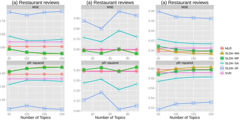
Figure 4: Performance ofSLDAusing different averaging strategies computed at the final training iterationTTR, compared with two baselinesMLRandSVR. Methods using multiple test chains (MFandMA) perform as well as or better than the two baselines, whereas methods using a single test chain (SFandSA) perform significantly worse.

Experimental setup: We use the same data as in Sec-tion 3. For all datasets, the metadata are the review rating, ranging from 1 to 5 stars, which is

standard-ized using z-normalization. We use two evaluation

metrics: mean squared error (MSE) and predictive

R-squared (Blei and McAuliffe, 2007).

For comparison, we consider two baselines: (1) multi-ple linear regression (MLR), which models the metadata

as a linear function of the features, and (2) support

vec-tor regression (Joachims, 1999,SVR). Both baselines

use the normalized frequencies of unigrams and bigrams as features. As in the unsupervised case, we report av-erage performance over five cross-validated folds. For all models, we use a development set to tune their pa-rameter(s) and use the set of parameters that gives best results on the development data at test.5

Results: Figure 3 showsSLDAprediction results with

different averaging strategies, computed at different training iterations.6 _{Consistent with the unsupervised}

results in Section 3,SA outperformsSF, but both are

outperformed significantly by the two methods using multiple test chains (MFandMA).

We also compare the performance of the four pre-diction methods obtained at the final iterationTTR of the training chain with the two baselines. The results in Figure 4 show that the two baselines (MLRandSVR)

out-perform significantly theSLDAusing only a single test 5_{ForMLRwe use a Gaussian priorN(0,1/λ)withλ=}

a·10b _{wherea ∈ [1,9]andb ∈ [1,4]; for SVR, we use}

SVMlight _{(Joachims, 1999) and varyC ∈ [1,50], which}

trades off between training error and margin; forSLDA, we fix

σ= 10and varyρ∈ {0.1,0.5,1.0,1.5,2.0}, which trades off between the likelihood of words and response variable.

6_{MCMC setup: T}

TR = 5,000 for RESTAURANT and MOVIEand1,000for HOTEL; for all datasetsBTR = 500,

LTR= 50,TTE= 100,BTE= 20andLTE= 5.

chains (SFandSA). Methods using multiple test chains

(MFandMA), on the other hand, match the baseline7

(HOTEL) or do better (RESTAURANTand MOVIE).

5 Discussion and Conclusion

MCMCrelies on averaging multiple samples to

approxi-mate target densities. When used for prediction,MCMC

needs to generate and average over both training sam-ples to learn from training data and test samsam-ples to make prediction. We have shown that simple averaging—not more aggressive,ad hocapproximations like taking the final sample (either training or test)—is not just a ques-tion of theoretical aesthetics, but an important factor in obtaining good prediction performance.

Compared withSVRandMLRbaselines,SLDAusing

multiple test chains (MFandMA) performs as well as

or better, whileSLDAusing a single test chain (SFand SA) falters. This simple experimental setup choice can

determine whether a model improves over reasonable baselines. In addition, better prediction with shorter training is possible with multiple test chains. Thus, we conclude that averaging using multiple chains produces above-average results.

Acknowledgments

We thank Jonathan Chang, Ke Zhai and Mohit Iyyer for helpful discussions, and thank the anonymous reviewers for insightful comments. This research was supported in part by NSF under grant #1211153 (Resnik) and #1018625 (Boyd-Graber and Resnik). Any opinions, findings, conclusions, or recommendations expressed here are those of the authors and do not necessarily reflect the view of the sponsor.

7_{This gap is becauseSLDAhas not converged after 1,000}

References

Christophe Andrieu, Nando de Freitas, Arnaud Doucet, and Michael I. Jordan. 2003. An introduction to MCMC for machine learning.Machine Learning, 50(1-2):5–43. Arthur Asuncion, Max Welling, Padhraic Smyth, and

Yee Whye Teh. 2009. On smoothing and inference for topic models. InUAI.

David M. Blei and Jon D. McAuliffe. 2007. Supervised topic models. InNIPS.

David M. Blei, Andrew Ng, and Michael Jordan. 2003. Latent Dirichlet allocation.JMLR, 3.

David M. Blei. 2012. Probabilistic topic models. Commun. ACM, 55(4):77–84, April.

David M. Blei. 2014. Build, compute, critique, repeat: Data analysis with latent variable models. Annual Review of Statistics and Its Application, 1(1):203–232.

Jordan Boyd-Graber and Philip Resnik. 2010. Holistic sen-timent analysis across languages: Multilingual supervised latent Dirichlet allocation. InEMNLP.

Jonathan Chang. 2012. lda: Collapsed Gibbs sampling meth-ods for topic models. http://cran.r-project.

org/web/packages/lda/index.html. [Online;

accessed 02-June-2014].

Qixia Jiang, Jun Zhu, Maosong Sun, and Eric P. Xing. 2012. Monte Carlo methods for maximum margin supervised topic models. InNIPS.

Yohan Jo and Alice H. Oh. 2011. Aspect and sentiment unification model for online review analysis. InWSDM. Thorsten Joachims. 1999. Making large-scale SVM learning

practical. InAdvances in Kernel Methods - Support Vector Learning, chapter 11. Cambridge, MA.

Simon Lacoste-Julien, Fei Sha, and Michael I. Jordan. 2008. DiscLDA: Discriminative learning for dimensionality re-duction and classification. InNIPS.

D. Liu and J. Nocedal. 1989. On the limited memory BFGS method for large scale optimization.Math. Prog. Radford M. Neal. 1993. Probabilistic inference using Markov

chain Monte Carlo methods. Technical Report CRG-TR-93-1, University of Toronto.

Viet-An Nguyen, Jordan Boyd-Graber, and Philip Resnik. 2012. SITS: A hierarchical nonparametric model using speaker identity for topic segmentation in multiparty con-versations. InACL.

Viet-An Nguyen, Jordan Boyd-Graber, and Philip Resnik. 2013. Lexical and hierarchical topic regression. InNeural Information Processing Systems.

Bo Pang and Lillian Lee. 2005. Seeing stars: Exploiting class relationships for sentiment categorization with respect to rating scales. InACL.

Daniel Ramage, David Hall, Ramesh Nallapati, and Christo-pher Manning. 2009. Labeled LDA: A supervised topic model for credit attribution in multi-labeled corpora. In EMNLP.

Daniel Ramage, Christopher D. Manning, and Susan Dumais. 2011. Partially labeled topic models for interpretable text mining. InKDD, pages 457–465.

Philip Resnik and Eric Hardisty. 2010. Gibbs sampling for the uninitiated. Technical Report UMIACS-TR-2010-04, University of Maryland. http://drum.lib.umd.edu//handle/1903/10058.

Michal Rosen-Zvi, Thomas L. Griffiths, Mark Steyvers, and Padhraic Smyth. 2004. The author-topic model for authors and documents. InUAI.

Sameer Singh, Michael Wick, and Andrew McCallum. 2012. Monte Carlo MCMC: Efficient inference by approximate sampling. InEMNLP, pages 1104–1113.

Mark Steyvers and Tom Griffiths. 2006. Probabilistic topic models. In T. Landauer, D. Mcnamara, S. Dennis, and W. Kintsch, editors,Latent Semantic Analysis: A Road to Meaning.Laurence Erlbaum.

Hanna M. Wallach, Iain Murray, Ruslan Salakhutdinov, and David Mimno. 2009. Evaluation methods for topic models. In Leon Bottou and Michael Littman, editors,ICML. Hanna M Wallach. 2008.Structured Topic Models for

Lan-guage. Ph.D. thesis, University of Cambridge.

Chong Wang, David Blei, and Li Fei-Fei. 2009. Simultaneous image classification and annotation. InCVPR.

Hongning Wang, Yue Lu, and Chengxiang Zhai. 2010. La-tent aspect rating analysis on review text data: A rating regression approach. InSIGKDD, pages 783–792. Jun Zhu, Amr Ahmed, and Eric P. Xing. 2009. MedLDA:

maximum margin supervised topic models for regression and classification. InICML.