Efficient kernels for sentence pair classification
Fabio Massimo Zanzotto
DISP
University of Rome “Tor Vergata” Via del Politecnico 1
00133 Roma, Italy [email protected]
Lorenzo Dell’Arciprete
University of Rome “Tor Vergata” Via del Politecnico 1
00133 Roma, Italy
Abstract
In this paper, we propose a novel class of graphs, the tripartite directed acyclic graphs (tDAGs), to model first-order rule feature spaces for sentence pair classifi-cation. We introduce a novel algorithm for computing the similarity in first-order rewrite rule feature spaces. Our algorithm is extremely efficient and, as it computes the similarity of instances that can be rep-resented in explicit feature spaces, it is a valid kernel function.
1 Introduction
Natural language processing models are generally positive combinations between linguistic models and automatically learnt classifiers. As trees are extremely important in many linguistic theories, a large amount of works exploiting machine learn-ing algorithms for NLP tasks has been developed for this class of data structures (Collins and Duffy, 2002; Moschitti, 2004). These works propose ef-ficient algorithms for determining the similarity among two trees in tree fragment feature spaces.
Yet, some NLP tasks such as textual entail-ment recognition (Dagan and Glickman, 2004; Dagan et al., 2006) and some linguistic theories such as HPSG (Pollard and Sag, 1994) require more general graphs and, then, more general al-gorithms for computing similarity among graphs. Unfortunately, algorithms for computing similar-ity among two general graphs in term of com-mon subgraphs are still exponential (Racom-mon and G¨artner, 2003). In these cases, approximated al-gorithms have been proposed. For example, the one proposed in (G¨artner, 2003) counts the num-ber of subpaths in common. The same happens for the one proposed in (Suzuki et al., 2003) that is applicable to a particular class of graphs, i.e. the hierarchical directed acyclic graphs. These algo-rithms do not compute the number of subgraphs
in common between two graphs. Then, these al-gorithms approximate the feature spaces we need in these NLP tasks. For computing similarities in these feature spaces, we have to investigate if we can define a particular class of graphs for the class of tasks we want to solve. Once we focused the class of graph, we can explore efficient similarity algorithms.
A very important class of graphs can be de-fined for tasks involving sentence pairs. In these cases, an important class of feature spaces is the one that represents first-order rewrite rules. For example, in textual entailment recognition (Da-gan et al., 2006), we need to determine whether a text T implies a hypothesisH, e.g., whether or not “Farmers feed cows animal extracts” entails “Cows eat animal extracts”(T1, H1). If we want to learn textual entailment classifiers, we need to exploit first-order rules hidden in training in-stances. To positively exploit the training instance “Pediatricians suggest women to feed newborns breast milk” entails “Pediatricians suggest that newborns eat breast milk” (T2, H2) for classify-ing the above example, learnclassify-ing algorithms should learn that the two instances hide the first-order rule
ρ = feedY Z → YeatZ . The first-order rule feature space, introduced by (Zanzotto and Moschitti, 2006), gives high performances in term of accuracy for textual entailment recognition with respect to other features spaces.
In this paper, we propose a novel class of graphs, the tripartite directed acyclic graphs (tDAGs), that model first-order rule feature spaces and, using this class of graphs, we introduce a novel algorithm for computing the similarity in first-order rewrite rule feature spaces. The possi-bility of explicitly representing the first-order fea-ture space as subgraphs of tDAGs makes the de-rived similarity function a valid kernel. With re-spect to the algorithm proposed in (Moschitti and Zanzotto, 2007), our algorithm is more efficient
and it is a valid kernel function.
The paper is organized as follows. In Sec. 2, we firstly describe tripartite directed acyclic graphs (tDAGs) to model first-order feature (FOR) spaces. In Sec. 3, we then present the related work. In Sec. 4, we introduce the similarity func-tion for these FOR spaces. This can be used as ker-nel function in kerker-nel-based machines (e.g., sup-port vector machines (Cortes and Vapnik, 1995)). We then introduce our efficient algorithm for com-puting the similarity among tDAGs. In Sec. 5, we analyze the computational efficiency of our algorithm showing that it is extremely more ef-ficient than the algorithm proposed in (Moschitti and Zanzotto, 2007). Finally, in Sec. 6, we draw conclusions and plan the future work.
2 Representing first-order rules and
sentence pairs as tripartite directed acyclic graphs
As first step, we want to define the tripartite di-rected acyclic graphs (tDAGs). This is an ex-tremely important class of graphs for the first-order rule feature spaces we want to model. We want here to intuitively show that, if we model first-order rules and sentence pairs astDAGs, de-termining whether or not a sentence pair can be unified with a first-order rewrite rule is a graph matching problem. This intuitive idea helps in determining our efficient algorithm for exploiting first-order rules in learning examples.
To illustrate the above idea we will use an ex-ample based on the above ruleρ= feedY Z → YeatZ and the above sentence pair(T1, H1). The rule ρ encodes the entailment relation of the verb to feed and the verb to eat. If represented over a syntactic interpretation, the rule has the fol-lowing aspect:
ρ1=
VP
VB
feed
NP Y NP Z → S
NP Y VP
VB
eat
NP Z
As in the case of feature structures (Carpenter, 1992), we can observe this rule as a graph. As we are not interested in the variable names but we need to know the relation between the right hand side and the left hand side of the rule, we can substitute each variable with an unlabelled node. We then connect tree nodes having variables with
VP
VB
feed
NP NP ·
·
S
NP VP
VB
eat
[image:2.595.307.526.65.129.2]NP
Figure 1:A simple rewrite rule seen as a graph
S
NP
DT
The
NN
farmer
VP
VB
feed
NP
NNS
cows
NP
NN
animal
NNS
extracts
·
·
·
S
NP
NNS
Cows
VP
VB
eat
NP
NN
animal
NNS
[image:2.595.303.526.159.239.2]extracts
Figure 2:A sample pair seen as a graph
the corresponding unlabelled node. The result is a graph as the one in Fig. 1. The variables Y and Z are represented by the unlabelled nodes between the trees.
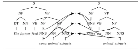
In the same way we can represent the sentence pair (T1, H1) using graph with explicit links be-tween related words and nodes (see Fig. 2). We can link words using anchoring methods as in (Raina et al., 2005). These links can then be prop-agated in the syntactic tree using semantic heads of the constituents (Pollard and Sag, 1994). The ruleρ1matches over the pair(T1, H1)if the graph
ρ1is among the subgraphs of the graph in Fig. 2.
Both rules and sentence pairs are graphs of the same type. These graphs are basically two trees connected through an intermediate set of nodes representing variables in the rules and relations be-tween nodes in the sentence pairs. We will here-after call these graphs tripartite directed acyclic graphs (tDAGs). The formal definition follows.
Definition tDAG: A tripartite directed acyclic
graph is a graphG= (N, E)where
• the set of nodesN is partitioned in three sets
Nt,Ng, andA
• the set of edges is partitioned in four setsEt,
Eg,EAt, andEAg
such thatt= (Nt, Et)andg = (Ng, Eg)are two trees andEAt ={(x, y)|x ∈ Ntandy ∈ A}and
EAg ={(x, y)|x ∈Ngandy ∈A}are the edges connecting the two trees.
The explicit representation of the tDAG in Fig. 2 has been useful to show that the unification of a rule and a sentence pair is a graph matching prob-lem. Yet, it is complex to follow. We will then de-scribe a tDAG with an alternative and more con-venient representation. A tDAG G = (N, E) can be seen as pair G = (τ, γ)of extended trees
τ and γ where τ = (Nt ∪ A, Et ∪ EAt) and
γ = (Ng ∪A, Eg ∪EAg). These are extended trees as each tree contains the relations with the other tree.
As for the feature structures, we will graphically represent a (x, y) ∈ EAt and a (z, y) ∈ EAg as boxes y respectively on the node x and on the node z. These nodes will then appear asL(x)y andL(z)y , e.g., NP 1 . The nameyis not a label but a placeholder representing an unlabelled node. This representation is used for rules and for sen-tence pairs. The sensen-tence pair in Fig. 2 is then represented as reported in Fig. 3.
3 Related work
Automatically learning classifiers for sentence pairs is extremely important for applications like textual entailment recognition, question answer-ing, and machine translation.
In textual entailment recognition, it is not hard to see graphs similar to tripartite directed acyclic graphs as ways of extracting features from exam-ples to feed automatic classifiers. Yet, these graphs are generally not tripartite in the sense described in the previous section and they are not used to ex-tract features representing first-order rewrite rules. In (Raina et al., 2005; Haghighi et al., 2005; Hickl et al., 2006), two connected graphs representing the two sentences s1 and s2 are used to compute distance features, i.e., features representing the distance betweens1 and s2. The underlying idea is that lexical, syntactic, and semantic similarities between sentences in a pair are relevant features to classify sentence pairs in classes such as entail and not-entail.
In (de Marneffe et al., 2006), first-order rewrite rule feature spaces have been explored. Yet, these spaces are extremely small. Only some features representing first-order rules have been explored. Pairs of graphs are used here to determine if a fea-ture is active or not, i.e., the rule fires or not. A larger feature space of rewrite rules has been im-plicitly explored in (Wang and Neumann, 2007) but this work considers only ground rewrite rules.
In (Zanzotto and Moschitti, 2006), tripartite di-rected acyclic graphs are implicitly introduced and exploited to build first-order rule feature spaces. Yet, both in (Zanzotto and Moschitti, 2006) and in (Moschitti and Zanzotto, 2007), the model pro-posed has two major limitations: it can represent rules with less than 7 variables and the proposed kernel is not a completely valid kernel as it uses the max function.
In machine translation, some methods such as (Eisner, 2003) learn graph based rewrite rules for generative purposes. Yet, the method presented in (Eisner, 2003) can model first-order rewrite rules only with a very small amount of variables, i.e., two or three variables.
4 An efficient algorithm for computing
the first-order rule space kernel
In this section, we present our idea for an effi-cient algorithm for exploiting first-order rule fea-ture spaces. In Sec. 4.1, we firstly define the simi-larity function, i.e., the kernelK(G1, G2), that we need to determine for correctly using first-order rules feature spaces. This kernel is strongly based on the isomorphism between graphs. A relevant idea of this paper is the observation that we can define an efficient way to detect the isomorphism between the tDAGs (Sec. 4.2). This algorithm ex-ploits the efficient algorithms of tree isomorphism as the one implicitly used in (Collins and Duffy, 2002). After describing the isomorphism between tDAGs, We can present the idea of our efficient al-gorithm for computingK(G1, G2)(Sec. 4.3). We introduce the algorithms to make it a viable solu-tion (Sec. 4.4). Finally, in Sec. 4.5, we report the kernel computation we compare against presented by (Zanzotto and Moschitti, 2006; Moschitti and Zanzotto, 2007).
4.1 Kernel functions over first-order rule feature spaces
The first-order rule feature space we want to model is huge. If we use kernel-based machine learning models such as SVM (Cortes and Vapnik, 1995), we can implicitly define the space by defining its similarity functions, i.e., its kernel functions. We firstly introduce the first-order rule feature space and we then define the prototypical kernel function over this space.
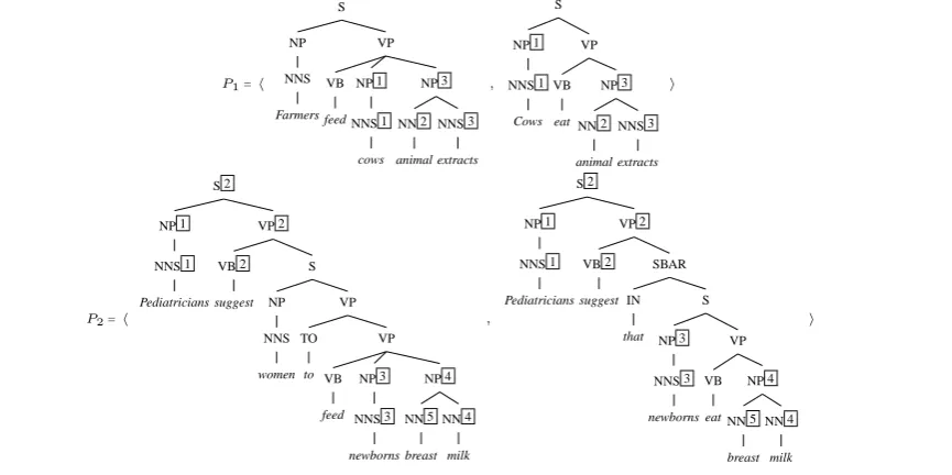
P1=h S NP NNS Farmers VP VB feed NP 1 NNS 1 cows NP 3 NN 2 animal NNS 3 extracts , S NP 1 NNS 1 Cows VP VB eat NP 3 NN 2 animal NNS 3 extracts i
P2=h
[image:4.595.94.527.64.280.2]S 2 NP 1 NNS 1 Pediatricians VP 2 VB 2 suggest S NP NNS women VP TO to VP VB feed NP 3 NNS 3 newborns NP 4 NN 5 breast NN 4 milk , S 2 NP 1 NNS 1 Pediatricians VP 2 VB 2 suggest SBAR IN that S NP 3 NNS 3 newborns VP VB eat NP 4 NN 5 breast NN 4 milk i
Figure 3: Two tripartite DAGs
rules defined as tDAGs. Within this space it is pos-sible to define the function S(G) that determines all the possible active features of the tDAGG in
F OR. The functionS(G)determines all the pos-sible and meaningful subgraphs of G. We want that these subgraphs represent first-order rules that can be matched with the pairG. Then, meaningful subgraphs ofG= (τ, γ)are graphs as(t, g)where
tandgare subtrees ofτ and γ. For example, the subgraphs ofP1andP2in Fig. 3 are hereafter par-tially represented:
S(P1)={ h S
NP VP
,
S
NP 1 VP
i,h NP 1 NNS 1 , NP 1 NNS 1 i, h S NP VP VB feed
NP 1 NP 3
,
S
NP 1 VP
VB eat NP 3 i, h VP VB feed
NP 1 NP 3 , S
NP 1 VP
VB
eat
NP 3
i, ...}
and
S(P2)={ h
S 2
NP 1 VP 2
,
S 2
NP 1 VP 2
i , h
NP 1 NNS 1 , NP 1 NNS 1 i , h VP VB feed
NP 3 NP 4 , S
NP 3 VP
VB
eat
NP 4
i, ...}
In the FOR space, the kernel functionKshould then compute the number of subgraphs in com-mon. The trivial way to describe the former kernel
function is using the intersection operator, i.e., the kernelK(G1, G2)is the following:
K(G1, G2) =|S(G1)∩ S(G2)| (1)
This is very simple to write and it is in principle correct. A graph g in the intersection S(G1) ∩
S(G2)is a graph that belongs to bothS(G1)and
S(G2). Yet, this hides a very important fact: de-termining whether two graphs, g1 and g2, are the same graph g1 = g2 is not trivial. For example, it is not sufficient to superficially compare graphs to determine that ρ1 belongs both to S1 and S2. We need to use the correct property for g1 = g2, i.e., the isomorphism between two graphs. We can call the operator Iso(g1, g2). When two graphs verify the property Iso(g1, g2), both g1 and g2 can be taken as the graph g representing the two graphs. Detecting Iso(g1, g2) has an exponential complexity (K ¨obler et al., 1993).
This complexity of the intersection operator be-tween sets of graphs deserves a different way to represent the operation. We will use the same sym-bol but we will use the prefix notation. The opera-tor is hereafter re-defined:
∩(S(G1),S(G2)) =
={g1|g1 ∈ S(G1),∃g2 ∈ S(G2), Iso(g1, g2)}
4.2 Isomorphism between tDAGs
We then observe that isomorphism between two tDAGs can be divided in two sub-problems:
• finding the isomorphism between two pairs of extended trees
• checking whether the partial isomorphism found between the two pairs of extended trees are compatible.
In general, two tDAGs, G1 = (N1, E1) and
G2 = (N2, E2) are isomorphic (or match) if
|N1| = |N2|, |E1| = |E2|, and a bijective func-tionf :N1 →N2exists such that these properties hold:
• for each noden∈N1,L(f(n)) =L(n)
• for each edge (n1, n2) ∈ E1 an edge (f(n1), f(n2))is inE2
The bijective functionfis a member of the combi-natorial setFof all the possible bijective functions between the two setsN1andN2.
The trivial algorithm for detecting if two graphs are isomorphic is exponential (K ¨obler et al., 1993). It explores all the set F. It is still unde-termined if the general graph isomorphism prob-lem is NP-complete. Yet, we can use the fact that tDAGs are two extended trees for building a bet-ter algorithm. There is an efficient algorithm for computing isomorphism between trees (as the one implicitly used in (Collins and Duffy, 2002)).
Given two tDAGs G1 = (τ1, γ1) and G2 = (τ2, γ2)the isomorphism problem can be divided in detecting two properties:
1. Partial isomorphism. Two tDAGsG1andG2 are partially isomorphic, ifτ1andτ2are iso-morphic and ifγ1andγ2are isomorphic. The partial isomorphism produces two bijective functionsfτ andfγ.
2. Constraint compatibility. Two bijective func-tionsfτ and fγare compatible on the sets of nodesA1andA2, if for eachn∈A1, it hap-pens thatfτ(n) =fγ(n).
We can rephrase the second property, i.e., the constraint compatibility, as follows. We de-fine two constraints c(τ1, τ2) and c(γ1, γ2) rep-resenting the functions fτ and fγ on the sets
A1 and A2. The two constraints are defined as
c(τ1, τ2) = {(n, fτ(n))|n∈A1}andc(γ1, γ2) =
{(n, fγ(n))|n ∈ A1}. Two partially isomorphic
tDAGs are isomorphic if the constraints match, i.e.,c(τ1, τ2) =c(γ1, γ2).
Pa= (τa, γa) =h
A 1
B 1
B 1 B 2 C 1
C 1 C 2
,
I 1
M 1
M 2 M 1 N 1
N 2 N 1
i
Pb= (τb, γb) =h
A 1
B 1
B 1 B 2 C 1
C 1 C 3
,
I 1
M 1
M 3 M 1 N 1
N 2 N 1
[image:5.595.319.513.60.157.2]i
Figure 5: Simple non-linguistic tDAGs
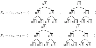
For example, the third pair of S(P1) and the second pair ofS(P2)are isomorphic as: (1) these are partially isomorphic, i.e., the right hand sides
τ and the left hand sides γ are isomorphic; (2) both pairs of extended trees generate the constraint
c1 = {(1,3),(3,4)}. In the same way, the fourth pair of S(P1) and the third pair of S(P2) generatec2={(1,1)}
4.3 General idea for an efficient kernel function
As above discussed, two tDAGs are isomorphic if the two properties, the partial isomorphism and the constraint compatibility, hold. To compute the kernel functionK(G1, G2)defined in Sec. 4.1, we can exploit these properties in the reverse order. Given a constraint c, we can select all the graphs that meet the constraint c(constraint compatibil-ity). Having the two set of all the tDAGs meeting the constraint, we can detect the partial isomor-phism. We split each pair of tDAGs in the four extended trees and we determine if these extended trees are compatible.
We introduce this innovative method to com-pute the kernel K(G1, G2) in the FOR space in two steps. Firstly, we give an intuitive explanation and, secondly, we formally define the kernel.
4.3.1 Intuitive explanation
To give an intuition of the kernel computation, without loss of generality and for sake of simplic-ity, we use two non-linguistic tDAGs,Pa and Pb (see Fig. 5), and the subgraph functionSe(θ). This latter is an approximated version ofS(θ)that gen-erates tDAGs with subtrees rooted in the root of the initial trees ofθ.
∩(Se(Pa),Se(Pb))|c1 = { h
A 1
B 1 C 1
,
I 1
M 1 N 1
i , h
A 1
B 1
B 1 B 2 C 1 ,
I 1
M 1 N 1
i , h
A 1
B 1
B 1 B 2 C 1 ,
I 1
M 1 N 1
N 2 N 1
i ,
h
A 1
B 1 C 1
,
I 1
M 1 N 1
N 2 N 1
i }={
A 1
B 1 C 1 ,
A 1
B 1
B 1 B 2
C 1 } × { I 1
M 1 N 1 ,
I 1
M 1 N 1
N 2 N 1
}=
=∩(Se(τa),Se(τb))|c1× ∩(Se(γa),Se(γb))|c1
∩(Se(Pa),Se(Pb))|c2 = { h
A 1
B 1 C 1
,
I 1
M 1 N 1
i , h
A 1
B 1 C 1
C 1 C 2
,
I 1
M 1 N 1
i , h
A 1
B 1 C 1
C 1 C 2
,
I 1
M 1
M 2 M 1
N 1 i ,
h
A 1
B 1 C 1
,
I 1
M 1
M 2 M 1
N 1 i }={
A 1
B 1 C 1 ,
A 1
B 1 C 1
C 1 C 2
} × {
I 1
M 1 N 1 ,
I 1
M 1
M 2 M 1
N 1 }=
=∩(Se(τa),Se(τb))|c2× ∩(Se(γa),Se(γb))|c2
Figure 4: Intuitive idea for the kernel computation
{(1,1),(2,2)},{(1,1),(2,3)} . We can then determine the kernelK(Pa, Pb)as:
K(Pa,Pb)= |∩(Se(Pa),Se(Pb))|=
= |∩(Se(Pa),Se(Pb))|c1S∩(Se(Pa),Se(Pb))|c2|
where ∩(Se(Pa),Se(Pb))|c are the common sub-graphs that meet the constraint c. A tDAGg0 = (τ0, γ0)inSe(P
a)is in∩(Se(Pa),Se(Pb))|c ifg00 =
(τ00, γ00)inSe(Pb)exists,g0 is partially isomorphic tog00, andc0 =c(τ0, τ00) =c(γ0, γ00)is covered by and compatible with the constraint c, i.e.,c0 ⊆c. For example in Fig. 4, the first tDAG of the set
∩(Se(Pa),Se(Pb))|c1 belongs to the set as its
con-straintc0 ={(1,1)}is a subset ofc1.
Observing the kernel computation in this way is important. Elements in ∩(Se(Pa),Se(Pb))|c already satisfy the property of constraint com-patibility. We only need to determine if the partially isomorphic properties hold for elements in ∩(Se(Pa),Se(Pb))|c. Then, we can write the following equivalence:
∩(Se(Pa),Se(Pb))|c=
[image:6.595.76.550.60.288.2]=∩(Se(τa),Se(τb))|c×∩(Se(γa),Se(γb))|c (2)
Figure 4 reports this equivalence for the two sets derived using the constraints c1 and c2. Note that this equivalence is not valid if a con-straint is not applied, i.e., ∩(Se(Pa),Se(Pb))
6
= ∩(Se(τa),Se(τb)) × ∩(Se(γa),Se(γb)).
The pair Pa itself does not belong to
∩(Se(Pa),Se(Pb)) but it does belong to
∩(Se(τa),Se(τb))× ∩(Se(γa),Se(γb)).
The equivalence (2) allows to compute the car-dinality of∩(Se(Pa),Se(Pb))|c using the cardinal-ities of ∩(Se(τa),Se(τb))|c and ∩(Se(γa),Se(γb))|c. These latter sets contain only extended trees where the equivalences between unlabelled nodes are given by c. We can then compute the cardinali-ties of these two sets using methods developed for trees (e.g., the kernel function KS(θ1, θ2) intro-duced in (Collins and Duffy, 2002)).
4.3.2 Formal definition
Given the idea of the previous section, it is easy to demonstrate that the kernel K(G1, G2)can be written as follows:
K(G1,G2)=|Sc∈C∩(S(τ1),S(τ2))|c×∩(S(γ1),S(γ2))|c|
where C is set of alternative constraints and
∩(S(θ1),S(θ2))|c are all the common extended
trees compatible with the constraintc.
We can compute the above kernel using the inclusion-exclusion property, i.e.,
|A1∪ · · · ∪An|=
X
J∈2{1,...,n}
(−1)|J|−1|A J| (3)
where 2{1,...,n} is the set of all the subsets of
{1, . . . , n}andAJ =Ti∈JAi.
To describe the application of the inclusion-exclusion model in our case, let firstly define:
whereθ1can be bothτ1andγ1andθ2can be both
τ2 andγ2. Trivially, we can demonstrate that:
K(G1, G2) =
=PJ∈2{1,...,|C|}(−1)|J|−1KS(τ1,τ2,c(J))KS(γ1,γ2,c(J))
(5)
wherec(J) =Ti∈Jci.
Given the nature of the constraint set C, we can compute efficiently the previous equation as it often happens that two different J1 and J2 in 2{1,...,|C|}generate the samec, i.e.
c= \
i∈J1
ci =
\
i∈J2
ci (6)
Then, we can defineC∗ as the set of all intersec-tions of constraints in C, i.e. C∗ = {c(J)|J ∈ 2{1,...,|C|}}. We can rewrite the equation as:
K(G1, G2) =
= X
c∈C∗
KS(τ1, τ2, c)KS(γ1, γ2, c)N(c) (7)
where
N(c) = X
J∈2{1,...,|C|}
c=c(J)
(−1)|J|−1 (8)
The complexity of the above kernel strongly de-pends on the cardinality ofCand the related cardi-nality ofC∗. The worst-case computational com-plexity is still exponential with respect to the size ofA1 and A2. Yet, the average case complexity (Wang, 1997) is promising.
The set C is generally very small with re-spect to the worst case. If F(A1,A2) are all the possible correspondences between the nodes
A1 and A2, it happens that |C| << |F(A1,A2)|
where|F(A1,A2)|is the worst case. For example, in the case of P1 and P2, the cardinality of
C = {(1,1)},{(1,3),(3,4),(2,5)} is extremely smaller than the one of
F(A1,A2) = {{( 1 , 1 ),( 2 , 2 ),( 3 , 3 )}, {( 1 , 2 ),( 2 , 1 ),( 3 , 3 )}, {( 1 , 2 ),( 2 , 3 ),( 3 , 1 )}, ...,{( 1 , 3 ),( 2 , 4 ),( 3 , 5 )}}. In Sec. 4.5 we argue that the algorithm presented in (Moschitti and Zanzotto, 2007) has the worst-case complexity.
Moreover, the setC∗ is extremely smaller than 2{1,...,|C|}due to the above property (6).
We will analyze the average-case complex-ity with respect to the worst-case complexcomplex-ity in Sec. 5.
4.4 Enabling the efficient kernel function
The above idea for computing the kernel function is extremely interesting. Yet, we need to make it viable by describing the way we can determine ef-ficiently the three main parts of the equation (7): 1) the set of alternative constraintsC(Sec. 4.4.1); 2) the set C∗ of all the possible intersections of constraints in C (Sec. 4.4.2); and, finally, 3) the numbersN(c)(Sec. 4.4.3).
4.4.1 Determining the set of alternative constraints
The first step of equation (7) is to determine the alternative constraints C. We can here strongly use the possibility of dividing tDAGs in two trees. We build C as Cτ ∪Cγ where: 1) Cτ are the constraints obtained from pairs of isomorphic ex-tended treest1∈ S(τ1)andt2 ∈ S(τ2); 2)Cγ are the constraints obtained from pairs of isomorphic extended treest1 ∈ S(γ1)andt2 ∈ S(γ2).
The idea for an efficient algorithm is that we can compute the C without explicitly looking at all the subgraphs involved. We instead use and combine the constraints derived comparing the productions of the extended trees. We can compute then Cτ with the productions of τ1 and
τ2 and Cγ with the productions of γ1 and γ2. For example (see Fig. 3), focusing on the τ, the rule NP3 → NN2NNS3 of G1 and
NP4 → NN5NNS4 ofG2generates the constraintc={(3,4),(2,5)}.
Using the above intuition it is possible to define an algorithm that builds an alternative constraint setCwith the following two properties:
1. for each common subtree according to a set of constraintsc,∃c0 ∈Csuch thatc⊆c0;
2. @c0, c00∈Csuch thatc0 ⊂c00andc06=∅.
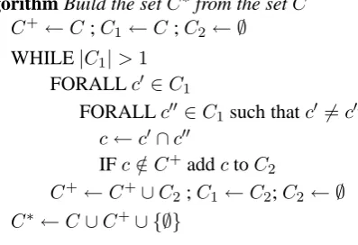
4.4.2 Determining the setC∗
The setC∗ is defined as the set of all possible in-tersections of alternative constraints inC. Figure 6 presents the algorithm determining C∗. Due to the property (6) discussed in Sec. 4.3, we can em-pirically demonstrate that the average complexity of the algorithm is not bigger than O(|C|2). Yet, again, the worst case complexity is exponential.
4.4.3 Determining the values ofN(c)
Algorithm Build the setC∗from the setC
C+←C;C
1 ←C;C2 ← ∅ WHILE|C1|>1
FORALLc0 ∈C1
FORALLc00∈C1such thatc0 6=c00
c←c0∩c00
IFc /∈C+addctoC2
C+←C+∪C
2;C1 ←C2;C2 ← ∅
[image:8.595.310.514.63.249.2]C∗←C∪C+∪ {∅}
Figure 6: Algorithm for computingC∗
the corresponding addend. It is possible to demon-strate that:
N(c) = 1− X
c0∈C∗
c0⊃c
Nc0 (9)
This recursive formulation of the equation allows us to easily determine the value ofN(c)for every
cbelonging toC∗. It is possible to prove this prop-erty using set properties and the binomial theorem. The proof is omitted for lack of space.
4.5 Reviewing the strictly related work
To understand if ours is an efficient algorithm, we compare it with the algorithm presented by (Mos-chitti and Zanzotto, 2007). We will hereafter call this algorithm Kmax. The Kmax algorithm and kernel is an approximation of what is a kernel needed for a FOR space as it is not difficult to demonstrate that Kmax(G1, G2) ≤ K(G1, G2). The Kmax approximation is based on maximiza-tion over the set of possible correspondences of the placeholders. Following our formulation, this kernel appears as:
Kmax(G1, G2) =
= max
c∈F(A1,A2)KS(τ1, τ2, c)KS(γ1, γ2, c)
(10)
where F(A1,A2) are all the possible correspon-dences between the nodesA1 and A2 of the two tDAGs as the one presented in Sec. 4.3. This for-mulation of the kernel has the worst case complex-ity of our formulation, i.e., Eq. 7.
For computing the basic kernel for the extended trees, i.e. KS(θ1, θ2, c) we use the model algo-rithm presented by (Zanzotto and Moschitti, 2006) and refined by (Moschitti and Zanzotto, 2007) based on the algorithm for tree fragment feature
0 10 20 30 40 50
0 10 20 30 40 50
ms
n×mplaceholders
[image:8.595.88.287.65.201.2]K(G1, G2) Kmax(G1, G2)
Figure 7: Mean execution time in milliseconds (ms) of the two algorithms wrt. n×m where n and mare the number of placeholders of the two tDAGs
spaces (Collins and Duffy, 2002). As we are using the same basic kernel, we can empirically compare the two methods.
5 Experimental evaluation
In this section we want to empirically estimate the benefits on the computational cost of our novel al-gorithm with respect to the alal-gorithm proposed by (Moschitti and Zanzotto, 2007). Our algorithm is in principle exponential with respect to the set of alternative constraints C. Yet, due to what pre-sented in Sec. 4.4 and as the set C∗ is usually very small, the average complexity is extremely low. Following the theory on the average-cost computational complexity (Wang, 1997), we es-timated the behavior of the algorithms on a large distribution of cases. We then compared the com-puting times of the two algorithms. Finally, as
K and Kmax compute slightly different kernels, we compare the accuracy of the two methods. We implemented both algorithmsK(G1, G2)and
Kmax(G1, G2) in support vector machine classi-fier (Joachims, 1999) and we experimented with both implementations on the same machine. We hereafter analyze the results in term of execution time (Sec. 5.1) and in term of accuracy (Sec. 5.2).
5.1 Average computing time analysis
0 200 400 600 800 1000 1200 1400 1600
0 2 4 6 8 10 12 14 s
[image:9.595.321.511.62.104.2]#ofplaceholders K(G1, G2) Kmax(G1, G2)
Figure 8: Total execution time in seconds (s) of the training phase on RTE2 wrt. different numbers of allowed placeholders
2006). The dataset of the challenge has 1,600 sen-tence pairs.
The computational cost of bothK(G1, G2)and
Kmax(G1, G2) depends on the number of place-holders n = |A1|of G1 and on m = |A2| the number of placeholders of G2. Then, in the first experiment we want to determine the relation be-tween the computational time and the factorn×m. Results are reported in Fig. 7 where the computa-tion times are plotted with respect ton×m. Each point in the curve represents the average execu-tion time for the pairs of instances havingn×m placeholders. As expected, the computation of the functionKis more efficient than the computation
Kmax. The difference between the two execution
times increases withn×m.
We then performed a second experiment that wants to determine the relation of the total exe-cution with the maximum number of placeholders in the examples. This is useful to estimate the be-havior of the algorithm with respect to its applica-tion in learning models. Using the RTE2 data, we artificially build different versions with increasing number of placeholders. We then have RTE2 with 1 placeholder at most in each pair, RTE2 with 2 placeholders, etc. The number of pairs in each set is the same. What changes is the maximal num-ber of placeholders. Results are reported in Fig. 8 where the execution time of the training phase in seconds (s) is plotted for each different set. We see that the computation of Kmax is exponential with respect to the number of placeholders and
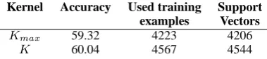
Kernel Accuracy Used training Support
examples Vectors
Kmax 59.32 4223 4206
[image:9.595.76.280.69.249.2]K 60.04 4567 4544
Table 1:Comparative performances ofKmaxandK
it becomes intractable after 7 placeholders. The computation of K is instead more flat. This can be explained as the computation of K is related to the real alternative constraints that appears in the dataset. The computation of the kernelKthen outperforms the computation of the kernelKmax.
5.2 Accuracy analysis
As Kmax that has been demonstrated very effec-tive in term of accuracy for RTE andK compute a slightly different similarity function, we want to show that the performance of our more computa-tionally efficientKis comparable, and even better, to the performances ofKmax. We then performed an experiment taking as training all the data de-rived from RTE1, RTE2, and RTE3, (i.e., 4567 training examples) and taking as testing RTE-4 (i.e., 1000 testing examples). The results are re-ported in Tab. 1. As the table shows, the accuracy ofK is higher than the accuracy ofKmax. There are two main reasons. The first is that Kmax is an approximation of K. The second is that we can now consider sentence pairs with more than 7 placeholders. Then, we can use the complete training set as the third column of the table shows.
6 Conclusions and future work
References
Roy Bar-Haim, Ido Dagan, Bill Dolan, Lisa Ferro, Danilo Giampiccolo, and Idan Magnini, Bernardo Szpektor. 2006. The second pascal recog-nising textual entailment challenge. In Proceedings
of the Second PASCAL Challenges Workshop on Recognising Textual Entailment. Venice, Italy.
Bob Carpenter. 1992. The Logic of Typed Fea-ture StrucFea-tures. Cambridge University Press,
Cam-bridge, England.
Michael Collins and Nigel Duffy. 2002. New rank-ing algorithms for parsrank-ing and taggrank-ing: Kernels over discrete structures, and the voted perceptron. In
Pro-ceedings of ACL02.
C. Cortes and V. Vapnik. 1995. Support vector net-works. Machine Learning, 20:1–25.
Ido Dagan and Oren Glickman. 2004. Probabilistic textual entailment: Generic applied modeling of lan-guage variability. In Proceedings of the Workshop
on Learning Methods for Text Understanding and Mining, Grenoble, France.
Ido Dagan, Oren Glickman, and Bernardo Magnini. 2006. The pascal recognising textual entailment challenge. In Quionero-Candela et al., editor, LNAI
3944: MLCW 2005, pages 177–190, Milan, Italy.
Springer-Verlag.
Marie-Catherine de Marneffe, Bill MacCartney, Trond Grenager, Daniel Cer, Anna Rafferty, and Christo-pher D. Manning. 2006. Learning to distinguish valid textual entailments. In Proceedings of the
Sec-ond PASCAL Challenges Workshop on Recognising Textual Entailment, Venice, Italy.
Jason Eisner. 2003. Learning non-isomorphic tree mappings for machine translation. In Proceedings
of the 41st Annual Meeting of the Association for Computational Linguistics (ACL), Companion Vol-ume, pages 205–208, Sapporo, July.
Thomas G¨artner. 2003. A survey of kernels for struc-tured data. SIGKDD Explorations.
Aria D. Haghighi, Andrew Y. Ng, and Christopher D. Manning. 2005. Robust textual inference via graph matching. In HLT ’05: Proceedings of the
con-ference on Human Language Technology and Em-pirical Methods in Natural Language Processing,
pages 387–394, Morristown, NJ, USA. Association for Computational Linguistics.
Andrew Hickl, John Williams, Jeremy Bensley, Kirk Roberts, Bryan Rink, and Ying Shi. 2006. Rec-ognizing textual entailment with LCCs GROUND-HOG system. In Bernardo Magnini and Ido Dagan, editors, Proceedings of the Second PASCAL
Recog-nizing Textual Entailment Challenge, Venice, Italy.
Springer-Verlag.
Thorsten Joachims. 1999. Making large-scale svm learning practical. In B. Schlkopf, C. Burges, and A. Smola, editors, Advances in Kernel
Methods-Support Vector Learning. MIT Press.
Johannes K¨obler, Uwe Sch ¨oning, and Jacobo Tor´an. 1993. The graph isomorphism problem: its
struc-tural complexity. Birkhauser Verlag, Basel,
Switzer-land, Switzerland.
Alessandro Moschitti and Fabio Massimo Zanzotto. 2007. Fast and effective kernels for relational learn-ing from texts. In Proceedlearn-ings of the International
Conference of Machine Learning (ICML). Corvallis,
Oregon.
Alessandro Moschitti. 2004. A study on convolution kernels for shallow semantic parsing. In
proceed-ings of the ACL, Barcelona, Spain.
C. Pollard and I.A. Sag. 1994. Head-driven Phrase
Structured Grammar. Chicago CSLI, Stanford.
Rajat Raina, Aria Haghighi, Christopher Cox, Jenny Finkel, Jeff Michels, Kristina Toutanova, Bill Mac-Cartney, Marie-Catherine de Marneffe, Manning Christopher, and Andrew Y. Ng. 2005. Robust tex-tual inference using diverse knowledge sources. In
Proceedings of the 1st Pascal Challenge Workshop,
Southampton, UK.
Jan Ramon and Thomas G¨artner. 2003. Expressivity versus efficiency of graph kernels. In First
Interna-tional Workshop on Mining Graphs, Trees and Se-quences.
Jun Suzuki, Tsutomu Hirao, Yutaka Sasaki, and Eisaku Maeda. 2003. Hierarchical directed acyclic graph kernel: Methods for structured natural language data. In In Proceedings of the 41st Annual
Meet-ing of the Association for Computational LMeet-inguis- Linguis-tics, pages 32–39.
Rui Wang and G¨unter Neumann. 2007. Recog-nizing textual entailment using a subsequence ker-nel method. In Proceedings of the Twenty-Second
AAAI Conference on Artificial Intelligence (AAAI-07), July 22-26, Vancouver, Canada.
Jie Wang. 1997. Average-case computational com-plexity theory. pages 295–328.
Fabio Massimo Zanzotto and Alessandro Moschitti. 2006. Automatic learning of textual entailments with cross-pair similarities. In Proceedings of the
21st Coling and 44th ACL, pages 401–408. Sydney,