Distributed energy storage using residential hot water heaters

Distributed Energy Storage Using Residential Hot

Water Heaters

Linas Gelažanskas * and Kelum A.A. Gamage

Engineering Department, Lancaster University, Bailrigg, Lancaster, LA1 4YW, UK; [email protected]

* Correspondence: [email protected]; Tel.: +37068210215

Abstract:This paper proposes and analyses a new demand response technique for renewable energy regulation using smart hot water heaters that forecast water consumption at an individual dwelling level. Distributed thermal energy storage has many advantages, including high overall efficiency, use of existing infrastructure and a distributed nature. In addition, the use of a smart thermostatic controller enables the prediction of required water amounts and keeps temperatures at a level that minimises user discomfort while reacting to variations in the electricity network. Three cases are compared in this paper, normal operation, operation with demand response and operation following the proposed demand response mechanism that uses consumption forecasts. The results show that this technique can produce both up and down regulation, as well as increase water heater efficiency. When controlling water heaters without consumption forecast, the users experience discomfort in the form of hot water shortage, but after the full technique is applied, the shortage level drops to nearly the starting point. The amount of regulation power from a single dwelling is also discussed in this paper.

Keywords:demand side management (DSM); distributed thermal storage; forecasting; water heater

1. Introduction

A distinctive characteristic of the electric power sector is that the amount of generated electricity has to be equal to the amount of consumed electricity at every single instance [1]. Unfortunately, there are peaks and valleys of total consumed electric energy, which do not always coincide with available generation patterns. People tend to have habits, including morning and evening rituals, that require large amounts of energy; thus, peaks are created. In addition, the generation side failures or other disruptions necessitate costly regulation ancillary services to match the demand with supply [2]. As a result, national transmission system operators (NTSO) constantly monitor the system and adjust the generation to meet the demand using ancillary services.

The increase of renewable energy generation attempts to solve problems associated with the conventional generation (such as emissions of greenhouse gasses), but creates power balancing issues [3]. Renewable energy is inherently intermittent and hard to control. As a result, its output is highly variable, and the electricity balancing problem becomes even more difficult [4]. Many researchers agree that wind generation introduces unprecedented amounts of uncertainty. The importance of demand side management (DSM) for long-term sustainable energy use in high renewable energy penetration areas is discussed in [5]. The power reserve limit needs to be increased when adding wind power to the system; otherwise, reliability is sacrificed [6]. It also makes unit commitment and economic dispatch problems more complicated, which are assessed in [7]. Studies show that in some countries in 2020, up to 13% of trade periods will require wind curtailment [8], indicating high wind generation uncertainty. According to [9], a forecasting horizon further than 4 h requires weather information to acquire better accuracy; therefore, wind generation forecasting results are highly dependant on the climate of a location. Wind power forecast uncertainty using probabilistic forecasting is described in [10], and in [6], the authors demonstrate the standard deviation of error of day-ahead forecast to be 0.22 per MW of installed power in Ireland. Up to now, traditional pumped hydro storage facilities primarily have served as part of the backup power,

but this cannot meet the high rate of output change from renewable power plants [2,11]. In addition, centralised backup power requires energy to be transmitted back and forth; thus, transmission losses have to be accounted for, as well.

Energy storage fundamentally improves the way electricity is generated, transmitted and consumed [12]. It allows the decoupling of generation from consumption to a certain level [13]. Hence, more storage on the grid significantly reduces generation dependency on the consumption. In addition, storage devices would also help during power outages, caused by equipment failures/faults or accidents. Moreover, the transmission and distribution grid has capacity limits, which might be exceeded during peak electricity usage. Energy storage would also help the grid to smooth energy transportation, increase electricity throughput to its maximum and increase load factor [14]. This would significantly lower the infrastructure costs as the transmission and distribution equipment has to be designed for peak demand, which occurs less than 5% of the time [3]. Furthermore, it enables the potential of running generating units at their maximum efficiency point, thus eventually decreasing generation costs.

DSM is a broad set of means to alter the time and magnitude of end user’s electricity consumption, one of which is load shifting. Load shifting techniques require storage capabilities, such as thermal storage devices. Water heaters are perfect candidates as demand responsive devices. In general, water heating accounts for 17% of all residential energy use in the United States [15]. Resistive hot water heaters are common in residential houses and make up 40% of all hot water heaters in the U.S. [15] and 12%–20% in the U.K. (depending on the season) [16], meaning the infrastructure is already established. They exhibit good thermal storage properties [17], possess high nominal power ratings and large thermal buffer capacities, as well as a fast response to load change [18–20]. Water has relatively high specific heat, which allows it to store large amounts of energy. Furthermore, in resistive water heaters, electricity is transferred to useful heat at 100% efficiency, and energy is lost only due to heat transfer through insulating walls.

Various hot water heater control techniques can be seen in the literature. The load commitment technique using real-time and forecasted pricing of electricity was researched by scientists in [21], whereas other researchers discussed a technique using timer switches for hot water load management [22]. Kepplingeret al.[23] demonstrate optimal control of hot water heaters using linear optimisation. The aggregate regulation service for renewable energy using thermally-stratified water heater model was analysed by Kondohet al.[24]. The model is designed to have two heating elements, but only one is assigned for regulation services; thus, in essence, only one half of the thermal capacity is used for demand response (DR), and the other half is used to guarantee end users’ comfort. Furthermore, there is an ongoing work to increase the efficiency of water heaters using baffles based on computational fluid dynamics [25]. Electric water heating control techniques to integrate wind power are compared by Fitzgerald et al. [26], whereas Finn et al. examines the impact of load scheduling on the adaption of wind generation [8]. Another study on the load balancing technique using an aggregate heating, ventilation and air conditioning (HVAC) system is presented by Lu in [27].

The widespread acceptance of DSM programs relies on minimal impact to the comfort of users [18]. This paper proposes a new strategy to control residential hot water heaters with minimal change in users’ comfort levels. In this research, the focus was to eliminate the imbalance caused by wind power plants, although this technique is not limited to solving problems associated with renewable energy generation. It could help in cases of generation faults or it could be used as an ancillary service or by energy traders to profit from the fluctuating real-time price of electricity.

2. System Description and Methodology

2.1. Thermal Water Heater Model

The dynamic thermal water heater model was derived based on open system energy balance [23,28,29]. The amount of energy consumed by the electric heating element is added to the model as an input, whereas the outputs are (1) energy consumed by hot water usage and (2) thermal energy losses due to imperfect thermal insulation. The amount of water drawn from the tank is based on measurement data collected from individual dwellings [30]. The temperature of the inlet water and the specific heat of water at normal temperature and pressure (NTP) conditions were also taken into account. Thermal losses are calculated based on the temperature difference between water and ambient temperature and thermal conductivity. The model is fully mixed, unstratified, meaning water temperature is the same throughout the tank. The effect of temperature variation at the output is compensated by demanding more water in case the temperature is cooler than the setpoint and demanding less if the temperature is higher. According to [31], the fully-mixed model shows increased thermal energy losses, so heat transfer coefficients were adjusted to compensate for this. Figure1graphically depicts the energy conservation of the system.

Figure 1.Thermal water heater diagram.

The mathematical model of the thermal system could be described as [28]:

Qt+1=Qt+∆tS0/1KHE+CWDt(TWH−Tin) +∆tk(TWH−Tamb) (1)

TWH= Qt

mCW

(2)

40◦C<TWH<90◦C (3)

whereQt(J) is the thermal energy stored in the water tank (integrator);∆t(s) is the time step length;

Figure 2.Thermal water heater block diagram model.

2.2. Smart Hot Water Heater Controller

The smart hot water heater controller in the proposed system controls the heating element according to the consumption forecasts and the signal sent from the smart grid. The controller is capable of locally forecasting hot water consumption of a particular dwelling. It contains an artificial neural network (ANN) model, which is trained based on the past hot water consumption information. The ANN model can compute short-term hot water usage forecasts tailored for the particular house. The controller also contains thermal model, so based on the consumption forecast, it can compute water temperature for the next 12 h period. It also receives a signal from the grid showing the requested duty cycle of the heating element. The signal is percentage-wise, where 0% means that the grid experiences a shortage of electricity, thus requesting to turn the heating element off, and 100% means a surplus of energy in the grid. The overall operation of the controller is described in Section2.5.

The ANN model that is used in the proposed system is based on the results from previous research [32,33]. In particular, a neural network nonlinear autoregressive exogenous (NARX) model is used. The configuration is the same as in Case #8 in [32] (p. 414). The ANN comprises an input layer, a single hidden layer consisting of 10 neurons and an output layer. The external inputs are the average consumption profile, as well as weekday and weekend dummy variables. The outputs of the ANN are fed back as inputs using a certain delay. It uses the Levenberg–Marquardt training algorithm, and the data are divided into training (15%), validation (15%) and test (70%) datasets. The training algorithm uses mean square error as the performance function to terminate the training. The overall performance of the model is summarised in Table1.

Table 1.Forecasting measures.

Measure Wind Generation Hot Water Consumption Forecast (per 1.5 kW) Forecast, kg

Mean 0.557 kW 6.145 kg

Standard deviation 0.374 kW 9.269 kg

Mean error −0.012 kW 0.042 kg

Standard deviation of error 0.137 kW 1.541 kg

Mean absolute error 0.099 kW 0.870 kg

Root mean square error 0.137 kW 1.548 kg

Normalised mean absolute error [33] 0.264 0.108

Normalised root mean square error [33] 0.368 0.192

The controller also implements temperature control. Despite any other factor, the controller attempts to maintain instantaneous temperature within the limits described in Equation (3). These are the upper and lower temperature safety bounds. If for any reason the temperature increased above 90◦C, it would disconnect the heating element until the temperature dropped below 88◦C. Similarly, if the temperature dropped below the critical 40◦C, it would turn on the heater regardless of the control signal from the system. This mechanism helps to ensure that the comfort level for the user is not impacted.

2.3. Wind Imbalance and Normal Consumption

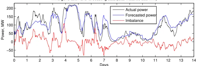
The performance of the system is assessed using previously-measured and -forecasted wind power generation data (total wind generation forecasts, as well as actual wind generation shown in Figure3) provided by the Lithuanian NTSO [34]. The overall goal of the newly-proposed DSM system is to create a backup power aggregator to cover forecasting error. The mismatch between forecast and actual generation can be either positive (surplus of energy) or negative (shortage of energy), and it is being referred to as the imbalance throughout the paper. Minimising imbalance enables renewable electricity sellers to supply the exact amount of electricity. The electricity that sells in the market can be delivered with high certainty, eliminating costly fines for under delivery of power or loss of income due to a lower price of unexpected energy generation (disconnection in the worst case). Table1contains statistical measures of the wind generation forecast data. The wind generation forecasts throughout the paper are based on the next day-ahead predictions to comprise the electricity day-ahead market. Furthermore, Table 1 presents hot water consumption forecast statistical information. It contains the arithmetic average of measures from all houses. These figures are calculated for one hour ahead forecasts.

0 1 2 3 4 5 6 7 8 9 10 11 12 13 14 −50

0 50 100 150 200

Wind generation and forecasting data (total installed 222 MW)

Power, MW

Days

Actual power Forecasted power Imbalance

Figure 3.Total actual and forecasted wind power.

0 1 2 3 4 5 6 7 8 9 10 11 12 13 14 −0.5

0 0.5 1 1.5

Normal water heater electricity consumption and wind imbalance

Power, kW

Days

Average normal consumption (water heater) Wind imbalance per 1.5 kW installed Power to be used by DSM (reference)

Figure 4. Average normal power consumption, wind power imbalance (fraction of 1.5 kW out of total 222 MW) and power to be used by the proposed demand side management (DSM) system per household.

2.4. Model Parameters and Assumptions

Modelling such a complex system required the careful selection of parameters, including temperature setpoints, sizes of the tanks, heating element ratings, ambient temperatures, thermal conductivity of the hot water tank, inlet water temperature,etc. One of the most important parameters in the context of energy accumulation is hot water tank volume. It describes how long a user can last without using electrical energy (in case of a shortage) or how much excessive electrical energy can be stored (in case of a surplus). In this paper, the hot water tanks were sized between 85 L and 200 L taking into account the average water consumption rate for a particular dwelling. Randomly-picked tank sizes from the chosen range were sorted in ascending order. The highest volume tank was matched to the dwelling with the most hot water consumption, and vice versa. Another crucial parameter of water heating devices is the rated power, where it defines how fast the electric energy is transferred to heat. From a demand response point of view, it is important during the times of energy surplus. The heating element power ratings were chosen to fall in a range from 1.5 kW to 2.5 kW [16]. The relationship of tank volume and heating elements can be seen in Figure5.

80 100 120 140 160 180 200

1.6 1.8 2 2.2 2.4

Tank volume and heating element relationship

Heating element rating, kW

Tank volume, liters

Figure 5.Water heater tank size and heating element power rating relationship.

2.5. Proposed Demand Side Management System Overall Operation

The main goal of the proposed system is to compensate day-ahead wind generation forecast errors. It enables the supply of the exact amount of wind energy that was sold in the day-ahead market and avoids charges for costly regulation ancillary services. At first, the forecast error is calculated by subtracting the day-ahead forecast from the actual wind generation. This is the power to be regulated using DR. Since water heaters can only consume electricity (regulate down), the imbalance is added on top of the predicted normal consumption to enable up regulation. The predicted normal water heater consumption information can be taken from the distribution system operator or, in this paper, it is modelled by the same ANN. Secondly, the actual electricity usage is aggregated and subtracted from the reference load. It is then used by the demand response controller to compute the request signal for the water heaters, which in turn decides whether to participate in the DR or not. Every 5 min, the controller forecasts individual demand for the next 12 h and computes the ability to participate in the demand response. It is only necessary to forecast 12 h ahead, because it takes about the same amount of time to raise the temperature by 50 degrees for a 200 L tank using a 1.5 kW heating element. Then, the controller computes the worst case scenario and checks whether the temperature is maintained in between the boundaries of comfort. The worst case scenario is achieved by turning the heater off for 5 min and when leaving it to work according to the thermostat. In the case of participation, the water heater reacts to the request signal and alters the energy use accordingly. As a result, the wind forecast error ends up balanced.

The simulation framework comprises 95 dwellings equipped with resistive hot water heater models of different sizes and power ratings, as well as 95 ANN models for every dwelling. The overall system diagram can be seen in Figure6.

Figure 6.Overall diagram of the system.

3. Results and Discussion

Finally, Case #3 depicts the proposed DSM with forecasting and the method of looking ahead. All values are per household.

Table 2.Performance measures.

Case Mean Power Mean Absolute Mean Mean Shortage Participation,

Consumption, W Final Imbalance, W Losses, W Temperature,◦C (% of Time) %

#1 (N/A) 325.7 144.3 49.4 67.5 0.11 (N/A)

#2 (1.0 kW) 309.4 26.6 54.4 73.1 1.19 100.0

#2 (1.5 kW) 298.7 47.1 52.6 71.4 1.95 100.0

#2 (2.0 kW) 290.0 72.3 51.2 70.0 2.74 100.0

#3 (1.5 kW) 313.9 52.1 46.9 65.9 0.30 94.0

Performance measures used in Table2can be summarised as follows:

• Mean power consumption is calculated by simply taking the arithmetic mean of the consumption profile from all dwellings.

• Mean absolute final imbalance is the arithmetic average of final absolute imbalance values. Figures are scaled to be per household per 1.5 kW of installed wind power.

• Mean losses: arithmetic average of thermal losses per hot water heater. • Mean temperature: arithmetic average of water temperature inside tanks.

• Shortage: average percentage of time the demanded water temperature was not supplied. • Participation: the average percentage of time that each water heater was participating in DSM.

The only time they are not participating is when there is expected high future consumption of hot water; thus, the temperature was expected to drop below critical, so the controller disconnects the particular water heater from DSM (therefore, increasing/maintaining user comfort).

Figure7 shows the relation between the time of shortage of hot water and the tank volume (Case #3). Most dwellings have not experienced any hot water shortage during the simulated period. Houses that suffered from the lack of hot water at some point in time show no correlation between their the tank size. As a result, it can be concluded that the installed tank size does not dictate how suitable the house is for DSM participation.

80 100 120 140 160 180 200 0

2 4 6

Shortage of hot water and tank volume relationship

Time of shortage, %

Tank volume, liters

Figure 7.The relationship of water heater tank size and the percentage of time the users experienced a shortage of hot water.

prepared hot water is inadequate for the amount that is actually needed, the proposed look ahead mechanism forecasts the required amount of hot water and controls temperature in a more efficient way. The temperature inside the water reservoir is decreased during energy shortages, whereas at the times of surplus energy, the temperature is increased to store energy. In fact, user comfort was affected in Case #2, but after demand forecasting was applied, it got restored to nearly the same level (shortage in Table2). Ancillary balancing services become available at virtually no cost, because the users do not notice any major difference in hot water supply due to the correct amounts of hot water that are prepared using forecasting.

3.1. Limitations

The fact that a negative imbalance can only be compensated by shedding the load leads to a certain limitation. The maximum power that can be shed is equal to the cumulative power the residences would normally use minus the power needed to maintain critically low water temperatures. In this particular case, the hot water consumption profile has very distinctive daily and weekly patterns. The consumption profile does not always coincide with the wind generation imbalance, thus during the valleys of normal energy consumption, there might be insufficient energy to be shed. Clearly, it can be expected that the proposed DSM mechanism will work best during peak hot water consumption periods and, hence, reduce the energy demand from the network. Figure8 demonstrates the average weekly consumption profile.

0 24 48 72 96 120 144 168

0 5 10 15

Mean hot water consumption profile

Mean consumption, kg

Hours

Mon Tue Wed Thu Fri Sat Sun

Figure 8.Weekly mean hot water consumption pattern [32].

0 100 200 300 400 500 600 700 800 900 1000 0

5 10 15 20 25

Power consumption and final wind imbalance relationship

Absolute final imbalance, kW

Normal consumption per household, W

Figure 9. Scatter diagram showing the relationship between normal consumption and final power imbalance.

7 8 9 10 11 12 13 14

−0.8 −0.6 −0.4 −0.2 0 0.2 0.4 0.6 0.8 1

Power usage and wind imbalance with and without DSM

Power, kW

Days Wind imbalance (1.5 kW)

Final system imbalance Normal power usage Power usage with DSM

Figure 10. Sample time plot showing alterations in power consumption and wind imbalance. The plot depicts results from Cases #1 and #3.

Another limitation is for the surplus energy,i.e., the maximum positive power imbalance the system can compensate. It is equal to the summed power rating of responsive water heaters (the ones with water temperatures below critically high) minus the forecasted normal consumption. In this paper, the normal consumption forecasts are computed using the same ANN models. As a result, every single dwelling cannot backup more installed power than its maximum rating, hence the chosen 1.5 kW value to be backed up by each dwelling. In addition, once the heater is fully charged (critical temperature reached) it is forced to the off state and cannot participate in DR. This creates vulnerability for long periods of surplus energy.

3.2. Temperatures

In case of hot water heater control using the DSM technique, without look ahead, there might be a situation where the temperature drops below a critical level. Such a situation occurs when an electricity shortage period is followed by substantial demand for hot water. The heating element is simply not capable of transferring heat at the same rate the water is drawn (otherwise, there would be no need for an accumulation tank). This case depicts a situation where the grid is satisfied by sacrificing user comfort (Case #2).

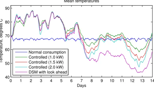
To overcome this problem, a control technique is added, which looks 12 h ahead and takes into account the forecasted consumption at every dwelling. Figure11depicts the average temperatures of normal consumption (i.e., the setpoint does not change), three DSM scenarios using different amounts of installed wind power to be balanced (per household) and average temperatures using the proposed DSM technique. It can be seen that using the traditional method, the temperature fluctuates around setpoint. In Case #2, three different amounts of backup power force the temperatures to swing in higher amplitudes, respectively. Finally, the mean temperature in Case #3 shows a different pattern, as there is a participation factor introduced to the system, which allows users to choose whether to participate in the DSM or not.

0 1 2 3 4 5 6 7 8 9 10 11 12 13 14 40

50 60 70 80 90

Mean temperatures

Temperature, degrees C

Days Normal consumption

Controlled (1.0 kW) Controlled (1.5 kW) Controlled (2.0 kW) DSM with look ahead

Figure 11.Sample average temperature time plot showing different simulation scenarios.

3.3. Losses

Thermal losses depend on the thermal conductivity coefficient of the tank walls and the difference in water and air temperatures. Since the thermal conductivity coefficient is constant and room temperature is also fairly constant, losses are mainly a function of temperature. Greater losses are experienced when water temperature is kept high. Therefore, in the event of shifting energy use into the future (delay raising the temperature), the heater exerts less heat waste, andvice versa. 3.4. Energy Balance

users were able to participate. The other 6% were notified by the tailored forecasting models that in case of participation there is a high chance of a hot water shortage. Therefore, user satisfaction was restored and the shortage percentage decreased. At the same time, Cases #2 and #3 demonstrate a decrease in final wind imbalance,i.e., wind generation variation was successfully backed up by the DSM technology. It should also be noticed that mean absolute final imbalance varied in Case #2 due to different amounts of installed wind power per household. The 1.5 kW per household of installed wind power has been observed to be optimal, as higher values cause the system to saturate and increase the final imbalance, which contradicts the key objective of this paper.

4. Conclusions

Due to the increased number of renewable energy sources, the electricity system requires more ancillary backup services every day. DSM techniques, such as distributed thermal energy storage using individual hot water heaters, can be utilised to tackle this problem. Forecasting hot water consumption at an individual level unveils each users needs; thus, the control can be applied such that the comfort is maintained at almost the same level. By having precise consumption forecasts, it is possible to prepare more accurate amounts of hot water compared to the functioning of a conventional water heater. At the same time, there is a wider margin for DSM operations. Using the proposed technique, time of water shortage increases from 0.11% to 0.3%. Compared to the results of Case #2 (1.95%), the increase in Case #3 is negligible. At the same time, the mean absolute final imbalance decreased by about 64%. The results confirm the initial hypothesis, that using such a DSM technique, it is possible to (1) lower the energy requirements for hot water preparation and (2) supply an ancillary service to the grid with minimal change in user comfort.

Acknowledgements: The authors would like to acknowledge the financial support of the Department of Engineering and Faculty of Science and Technology, Lancaster University, U.K., as well as the Energy Saving Trust for providing the necessary hot water consumption data.

Author Contributions: Linas Gelažanskas designed the models, performed simulations, and wrote the paper. Linas Gelažanskas and Kelum A.A. Gamage analyzed the data and corrected the paper.

Conflicts of Interest:The authors declare no conflict of interest.

References

1. Kundur, P.Power System Stability and Control; McGraw-Hill: Reading, MA, USA, 1994.

2. Baranauskas, A.; Gelažanskas, L.; Ažubalis, M.; Gamage, K. Control strategy for balancing wind power using hydro power and flow batteries. In Proceedings of the 2014 IEEE International Energy Conference (ENERGYCON), Cavtat, Croatia, 13–16 May 2014; pp. 352–357.

3. Gelažanskas, L.; Gamage, K.A. Demand side management in smart grid: A review and proposals for future direction. Sustain. Cities Soc.2014,11, 22–30.

4. Lund, P.D.; Lindgren, J.; Mikkola, J.; Salpakari, J. Review of energy system flexibility measures to enable high levels of variable renewable electricity. Renew. Sustain. Energy Rev.2015,45, 785–807.

5. Pina, A.; Silva, C.; Ferrao, P. The impact of demand side management strategies in the penetration of renewable electricity. Energy2012,41, 128–137.

6. Doherty, R.; O’Malley, M. A new approach to quantify reserve demand in systems with significant installed wind capacity. IEEE Trans. Power Syst.2005,20, 587–595.

7. Wang, J.; Botterud, A.; Bessa, R.; Keko, H.; Carvalho, L.; Issicaba, D.; Sumaili, J.; Miranda, V. Wind power forecasting uncertainty and unit commitment. Appl. Energy2011,88, 4014–4023.

8. Finn, P.; Fitzpatrick, C.; Connolly, D.; Leahy, M.; Relihan, L. Facilitation of renewable electricity using price based appliance control in Ireland’s electricity market. Energy2011,36, 2952–2960.

10. Matos, M.; Bessa, R. Setting the Operating Reserve Using Probabilistic Wind Power Forecasts.IEEE Trans. Power Syst.2011,26, 594–603.

11. Gelažanskas, L.; Baranauskas, A.; Gamage, K.A.; Ažubalis, M. Hybrid wind power balance control strategy using thermal power, hydro power and flow batteries. Int. J. Electr. Power Energy Syst. 2016, 74, 310–321.

12. Divya, K.; ßstergaard, J. Battery energy storage technology for power systems—An overview. Electr. Power Syst. Res.2009,79, 511–520.

13. Chen, H.; Cong, T.N.; Yang, W.; Tan, C.; Li, Y.; Ding, Y. Progress in electrical energy storage system: A critical review. Prog. Nat. Sci.2009,19, 291–312.

14. Denholm, P.; Sioshansi, R.The value of compressed air energy storage with wind in transmission-constrained electric power systems. Energy Policy2009,37, 3149–3158.

15. Hepbasli, A.; Kalinci, Y. A review of heat pump water heating systems. Renew. Sustain. Energy Rev.2009, 13, 1211–1229.

16. Newborough, M.; Augood, P. Demand-side management opportunities for the UK domestic sector. IEE Proc. Gener. Transm. Distrib.1999,146, 283–293.

17. Armstrong, P.; Ager, D.; Thompson, I.; McCulloch, M. Improving the energy storage capability of hot water tanks through wall material specification. Energy2014,78, 128–140.

18. Paull, L.; Li, H.; Chang, L. A novel domestic electric water heater model for a multi-objective demand side management program. Electr. Power Syst. Res.2010,80, 1446–1451.

19. Ericson, T. Direct load control of residential water heaters.Energy Policy2009,37, 3502–3512.

20. Vanthournout, K.; D’hulst, R.; Geysen, D.; Jacobs, G. A Smart Domestic Hot Water Buffer. IEEE Trans. Smart Grid2012,3, 2121–2127.

21. Du, P.; Lu, N. Appliance Commitment for Household Load Scheduling. IEEE Trans. Smart Grid2011, 2, 411–419.

22. Atikol, U. A simple peak shifting DSM (demand-side management) strategy for residential water heaters. Energy2013,62, 435–440.

23. Kepplinger, P.; Huber, G.; Petrasch, J. Autonomous optimal control for demand side management with resistive domestic hot water heaters using linear optimization. Energy Build.2015,100, 50–55.

24. Kondoh, J.; Lu, N.; Hammerstrom, D. An evaluation of the water heater load potential for providing regulation service. In Proceedings of the 2011 IEEE Power and Energy Society General Meeting, San Diego, CA, USA, 24–29 July 2011; pp. 1–8.

25. Sedeh, M.M.; Khodadadi, J. Energy efficiency improvement and fuel savings in water heaters using baffles. Appl. Energy2013,102, 520–533.

26. Fitzgerald, N.; Foley, A.M.; McKeogh, E. Integrating wind power using intelligent electric water heating. Energy2012,48, 135–143.

27. Lu, N. An Evaluation of the HVAC Load Potential for Providing Load Balancing Service. IEEE Trans. Smart Grid2012,3, 1263–1270.

28. Du, P.; Lu, N. Appliance Commitment for Household Load Scheduling. IEEE Trans. Smart Grid2011, 2, 411–419.

29. Nehrir, M.; Jia, R.; Pierre, D.; Hammerstrom, D. Power Management of Aggregate Electric Water Heater Loads by Voltage Control. In Proceedings of the 2007 IEEE Power Engineering Society General Meeting, Tampa, FL, USA, 24–28 June 2007; pp. 1–6.

30. Measurement of Domestic Hot Water Consumption in Dwellings; Technical Report; Energy Saving Trust: London, UK, 2008.

31. Celador, A.C.; Odriozola, M.; Sala, J. Implications of the modelling of stratified hot water storage tanks in the simulation ofCHPplants. Energy Convers. Manag.2011,52, 3018–3026.

33. Gelažanskas, L.; Gamage, K.A.A. Forecasting Hot Water Consumption in Residential Houses. Energies 2015,8, 12336.

34. Gelažanskas, L.; Gamage, K.A.Wind Generation; Data catalogue, Lancaster University Library, UK, 2015.

c