hare nonlinear functions,u is the input vector, wis



Abstract—In this paper, an adaptive constrained unscented Kalman filter (ACUKF) has been used for nonlinear structural system identification. The proposed algorithm takes into account state constraints and calculates online the measurement noise covariance matrix. The proposed method has been compared to the well-known unscented Kalman filter (UKF) for parameter estimation of a SDOF nonlinear hysteretic system. Numerical results show that the ACUKF is more robust to measurement noise level than the UKF, providing better state estimation and parameter identification.

Index Terms— Constrained unscented Kalman filter, Adaptive Kalman filter, Nonlinear system identification, Structural dynamics.

I.INTRODUCTION

The Kalman filter (KF) approach has been often adopted in several engineering applications to estimate the state of a given system from recorded measurements [1-4]. The unscented Kalman filter (UKF) is one of the KF-based algorithms widely adopted for the structural dynamics identification and there are numerous successfully applications of this method in literature [5, 6].

However, the application of UKF to highly nonlinear structural systems can provide not satisfactory results [7]. In this paper, the UKF algorithm has been improved with respect to two fundamental aspects: the ability to take into account state constraints and the ability to adaptively calculate the measurement noise covariance matrix.

The proposed adaptive constrained unscented Kalman filter (ACUKF) takes into account bounds of state variables and this is particularly useful as remediation for inaccurate system modelling which is often the case of real-world applications [7-9]. In addition, the ACUKF provides an adaptive identification of the measurement noise covariance matrix. It is well-known that an improper selection of process and measurement noise covariance matrices may cause a large estimation error or even the divergence of the whole system [10]. Generally, finding a suitable value of the process and measurement noise covariance matrices by the S. Strano is with the Department of Industrial Engineering, University of Naples Federico II, 80125 ITALY (corresponding author, phone: +390817683277; e-mail: salvatore.strano@unina.it).

M. Terzo is with the Department of Industrial Engineering, University of Naples Federico II, 80125 ITALY (e-mail: mario.terzo@unina.it).

classical method is time consuming. Moreover, measurement noise covariance can vary in actual application due to electromagnetic interference between sensors and other electrical instruments. The major function of the proposed adaptive algorithm is to get the measurement noise covariance matrix based on the filter learning history [10]. This allows to get better performance in the estimation. In this paper, the ACUKF and the UKF have been applied to a highly nonlinear hysteresis system based on the normalized Bouc-Wen model for the numerical evaluation of both methods. Several tests have been performed in order to investigate the robustness of the two techniques to the measurement noise level.

The paper is organized as follows: a description the ACUKF is given in Section 2. The mathematical particularization of the ACUKF for the nonlinear hysteresis model is given in Section 3. Simulation results are presented in Section 4.

II.ADAPTIVE CONSTRAINED KALMAN FILTER

Consider the following continuous nonlinear state space description with discrete measurements sampled at regular intervals with sampling period t





1 1 1 1

) 1 ( 1

) , (

), (

   

 

 

 

  

 



k k k k

k k t

k t

k k

k

k d (k t)

v u x h y

x x w u

x f x

x  

(1)

where _xRn _{is the n-dimensional vector of system state, f} and h are nonlinear functions, u is the input vector,w is the process noise with covariance

Q

, yRm is the m -dimensional vector of measurement,

v

is the Gaussian white measurement noise with covariance R and k is the k -th time step. The main task is to estimate -the system state, i.e., calculate the mean as well as the covariance of system state at the (k+1)-th step, based on the state estimation at the k-th step and the measurements at the current (k+1)-th step.

Given the filtered state estimates xˆk |k,which have been obtained using all the measurements made up to time tk, and the input u_k, the predicted state estimates xˆk1 |k can be obtained as



( ),



; ˆ ˆ ˆ

ˆ _{1 | |} ( 1) d k _|k (k t)

t k

t

k k

k k k

k  



 

 



 x f x u x x

x   . (2)

An Unscented Kalman Filter for Nonlinear

Hysteretic System Identification with State

Constraints and Adaptation of Measurement

Noise Covariance

In addition, bound constraints are imposed to the states as

U

L x x

x   (3) where xU and xL are the upper and lower bound of

constrained vectors, respectively.

Indicating with xˆk |kthe filtered state estimates at time instant ‘k’ and Pk |k the corresponding estimate error covariance matrix and denoting with







kk



_i k n i k k k i | , 1 | , P s P s     (4)

as the directions along which the sigma points are selected, according to the standard UKF, the step sizes for all sigma points, for the simple case when only bound constraints are considered, can be performed as follows [9]:

n i n i n i n n i j i k j i k j k k j L L i k j i k j i k j k k j U U i k L i k U i k C i k C i n k C i k i n k i k 2 , ... , 1 , 0 ) ( if , ) ( ) ˆ ( ) ( , min 2 , ... , 1 , 0 ) ( if , ) ( ) ˆ ( ) ( , min 2 , ... , 1 ), , , min( , ... , 1 ), , min( , , | , , , | , , , , , , , ,                                   s s x x θ s s x x θ θ θ θ θ θ θ θ  (5) where the subscript j represents the j-th element of the vector x. In the absence of bounds, the above choice of sigma points are identical to those used in UKF. If the current estimate is close to the bounds, then the above choice ensures that none of the sigma points violate the bounds on state variables. The weights of all of sigma points are adjusted by using a linear weighting method proposed in [11]: 2 , ... , 1 , 0 , , , 0 , n i b a i b i k i k k      θ W W

. (6)

where



              n i i k k k k s n n s n n b n n s n a 2 1 , . ] ) 1 2 ( [ 2 1 -2 ) 2( 1 ] ) 1 2 ( )[ 2( 1 -2 θ        (7)

The replacement of sigma points results in a first-order accuracy for the unscented transformation of mean value if

5 . 0



 , that is the value adopted in this paper.

Each sigma point Χk |k,i is transformed through the state-space equation in order to obtain sigma point of state prediction Χk1 |k,i, the mean of the predicted state estimate

k k 1 |

ˆ _

x and its error covariance matrix P_{k1 |k} , as well as the calculation of the predicted measurement sigma points

i k k1 | ,

Υ , the mean yˆ_{k1 |k} and covariance matrix k

k yy, 1 |

P

of predicted measurement and the cross covariance matrix

P

_{xy,k1 |k}, according to the standard UKF method.

The transformed sigma points are calculated with Kalman updating equation n i i k k k k i k k i k

k1 | 1, Χ 1 | , K 1(y 1Υ 1 | , ), 0,1 ,... ,2

Χ

(8) in accordance with the method proposed in [8].

With Χk1 |k1,i calculated by (8), the state update xˆk1 |k1

and its covariance Pk1 |k1 can be calculated using the

following equations: T 1 1 1 T 1 | 1 , 1 | 1 2 0 1 | 1 , 1 | 1 , 1 | 1 2 0 , 1 | 1 , 1 | 1 ) ˆ ( ) ˆ ( ˆ                          





k k k k k k i k k n i k k i k k i k k k n i i k k i k k k K R K Q x Χ x Χ W P Χ W x

. (9) It can be proved that the above equations give exactly the same result of updated mean and covariance with the standard UKF [7].

The adaptation of matrix R is described as follows:

) , ˆ ( ), 1 /( ) 1 ( ), ( 1 1 | 1 1 1 1 1 | 1 , T 1 1 1 1                     k k k k k k k k k yy k k k k k b b d d u x h y ε P ε ε R R (10)

where dk is a scaling parameter, b denotes a forgetting factor and usually between 0.95 and 0.995, and ek refers to the error between the actual measurement and the filter estimation in the kth step. Through the adaptive algorithm, the measurement noise covariance matrix can be computed step by step online [10]. Thus, the system estimation cannot be restricted by the initial noise covariance, and can adapt the variable system well.

III.SDOF NONLINEAR HYSTERETIC SYSTEM

Consider a single degree of freedom (SDOF) nonlinear hysteretic system subject to an acceleration input. The hysteresis force is mathematically described by the normalized Bouc-Wen model (NBWM) [12];

) ( ) ( ) ( )

(t cxt F t mx t x

m     _g (11)

where m is the mass, x(t) is the displacement, c is the linear viscous coefficient, F(t) is hysteretic component and

x



_g

(

t

)

          _{ }      

 () 1 () 1 sgn( () ( )) 1

) ( ) ( ) ( ) ( t w t u t w t u t w t w k t x k t F n w f  

 , (12)

where the parameters of the normalized form of the Bouc-Wen model are ρ, σ, n, kf, kw with the following constraints:

. 0 ; 0 ; 1 ; 2 1 ;

0    

  n k_f k_w

 (13)

Moreover, it is demonstrated that w(t) is bounded in the range [-1, 1] [13].

An augmented state vector x is defined as

                                                          n k k cw x x x x x x x x x x x w f    9 8 7 6 5 4 3 2 1 x . (14)

Then the state space equation is formulated based on (11) and (12) as fallows





                                                                                                                    0 0 0 0 0 0 1 ) sgn( 1 1 ) ( ), ( 8 3 1 8 3 1 7 1 6 3 4 1 5 2 9 8 7 6 5 4 3 2 1 9 x x x x x x x x m x x x x x x x n k k c w x x x x x x x x x x x t t x g w f                      u x f x (15) where u is the base excitation.

The derivatives of the NBWM parameters are all zero because they are assumed to be constant. A discrete time form of (15) is given by

k k k k k k k k k k k x k k k k k k k k k k k k g k k x x x x x x x x x x x t x x x tx x m x x x x x x x t x k w x                                                                           , 9 , 8 , 7 , 6 , 5 , 4 , 8 , 3 , 1 , 8 , 3 , 1 , 7 , 3 , 1 , 2 , 6 , 3 , 4 , 1 , 5 , 2 , 1 1 1 ) sgn( 1

1 9,



(16) where a process noise

w

has been added.

If the acceleration response and excitation are measured, the observation equation can be expressed as

v x x

y  _g , (17) where x is the acceleration of the suspended mass and v represents the measurement noise.

The function h (see (1) for reference) can be written as follows 1 1 , 6 1 , 3 1 , 4 1 , 1 1 , 5 1 , 2 1 1 1

1 ( , )

                  k k k k k k k k k k k v m x x x x x x v u x h y

. (18)

The bound constraints of the ACUKF are

1 , 2 1 , 0 , 0 , 0 , 0 , 1

1 3 4 5 6  7 8 9 

 x x x x x x x (19)

in accordance with (13) and considering that w(t) is bounded in the range [-1, 1]. Consequently, the application of the ACUKF to the NBWM is particular suitable to constrain both the parameter values and the state variable w, improving accuracy and robustness of the hysteresis estimation.

IV.SIMULATION TESTS

Simulations have been performed by assigning to the model previously described the Chi-Chi earthquake acceleration. The acceleration time history has a duration of 20 s with its maximum scaled value equal to 3 m/s2_.

Two white noises equal to 0.12 _m2_/s4 _{(TEST 1) and 0.2}2

m2_/s4 _{(TEST 2) have been superimposed to the simulated}

mass acceleration and the ground input acceleration, at t = 5 s for the purpose of exploring the identification robustness with respect to a sudden variation of the measurement noise. The ACUKF and the UKF have been parameterized in the same way and the initial value of R has been fixed to the measurement noise level before t = 5 s, equal to 0.012 _m2_/s4

Figs. 1-6 show the estimated parameters compared with the exact ones, for the TEST 1.

Fig. 1. Estimation of parameter c, TEST 1.

Fig. 2. Estimation of parameter kf, TEST 1.

Fig. 3. Estimation of parameter kw, TEST 1.

Fig. 4. Estimation of parameter ρ, TEST 1.

Fig. 5. Estimation of parameter σ, TEST 1.

Fig. 6. Estimation of parameter n, TEST 1.

The results clearly show that the ACUKF demonstrates a better robustness with respect to measurement noise level. Indeed, after a variation of R the parameters estimated with the ACUKF method are very close to exact ones. In contrast, the estimated parameters with the UKF degrades with the variation of R, as it is possible to note in the figures above.

Fig. 7 presents the estimation of the measurement noise my means of the ACUKF.

Fig. 7. Measurement covariance estimation with the ACUKF, TEST 1.

Fig. 8 shows the estimated displacements and exact one obtained by numerical integration.

Results of Fig. 8 highlight that the estimation error of the UKF is greater than the one of the ACUKF, especially after the sudden variation of the measurement noise.

The main results of TEST 2 are presented in the following. In this case, the measurement noise level is greater than the one of TEST 1.

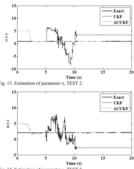
[image:5.595.308.530.51.330.2]

For comparison purpose, Figs. 9-14 show the estimated parameters compared with the exact ones, for the TEST 2.

[image:5.595.51.276.153.463.2]

Fig. 9. Estimation of parameter c, TEST 2.

[image:5.595.47.276.338.719.2]

Fig. 10. Estimation of parameter kf, TEST 2.

[image:5.595.309.531.447.574.2]

Fig. 11. Estimation of parameter kw, TEST 2.

Fig. 12. Estimation of parameter ρ, TEST 2.

Fig. 13. Estimation of parameter σ, TEST 2.

Fig. 14. Estimation of parameter n, TEST 2.

The UKF, after a variation of the measurement noise level (at t=5 s), provides poor results in terms of parameter estimation. For example, some parameters assume values out of their bounds without a physical meaning.

Estimated displacement diagrams presented in Fig. 15 clearly show the effectiveness of the ACUKF and the divergence of the UKF that cannot handle measurement noise variation.

Fig. 15. Suspended mass displacement estimation, TEST 2.

The estimation of the measurement noise my means of the ACUKF is shown in Fig. 16.

Fig. 16. Measurement covariance estimation with the ACUKF, TEST 2.

[image:5.595.312.535.630.744.2]

estimation practically superimposed to the exact one, also after a sudden variation of the measurement noise.

Simulation results show that the method ACUKF takes into account state constraints and it is robust to variations of R

due to its adaptive property.

V.CONCLUSION

The design of a novel adaptive constrained unscented Kalman filter (ACUKF) is presented in this paper. The performance of the ACUKF is compared with that one of the unscented Kalman filter (UKF) for a state estimation and the parameter identification applied to a SDOF nonlinear hysteretic system. The nonlinear behaviour has been mathematically described by the normalized Bouc-Wen model. The estimation capabilities and the robustness of both methods have been evaluated for different measurement noise levels. The numerical results have shown the ability of the ACUKF to identify a sudden variation of noise level, demonstrating its robustness. The ACUKF has provided more accurate estimation results than the UKF, also improving the convergence capability of the standard UKF. The ACUKF could be adopted in adaptive control methodologies where a real-time nonlinear system identification is required.

REFERENCES

[1] Majji, M., Junkins, J.L., Turner, J.D. (2010). A perturbation method for estimation of dynamic systems. Nonlinear Dynamics, 60 (3), 303-325.

[2] Calabrese, A., Strano, S., Serino, G., Terzo, M. (2014). An extended Kalman Filter procedure for damage detection of base-isolated structures. EESMS 2014 - 2014 IEEE Workshop on Environmental, Energy and Structural Monitoring Systems, Proceedings, art. no. 6923262, 40-45

[3] Calabrese, A., Strano, S., Terzo, M. (2016). Parameter estimation method for damage detection in torsionally coupled base-isolated structures. Meccanica, 51 (4), 785-797.

[4] Strano, S., Terzo, M. (2016). Actuator dynamics compensation for real-time hybrid simulation: an adaptive approach by means of a nonlinear estimator. Nonlinear Dynamics, 85 (4), 2353-2368. [5] Ntotsios, E., Karakostas, C., Lekidis, V., Panetsos, P., Nikolaou, I.,

Papadimitriou, C., Salonikos, T. (2010). Structural identification of Egnatia Odos bridges based on ambient and earthquake induced vibrations. Bulletin of Earthquake Engineering, 7, 485–501. [6] Xie, Z., Feng, J. (2012). Real-time nonlinear structural system

identification via iterated unscented Kalman filter. Mechanical Systems and Signal Processing, 28, 309-322.

[7] Wu, B., Wang, T. (2014). Model updating with constrained unscented Kalman filter for hybrid testing. Smart Structures and Systems, 14 (6), 1105-1129.

[8] Kolas, S., Foss, B. and Schei, T. (2009). Constrained nonlinear state estimation based on the UKF approach. Computers & Chemical Engineering, 33 (8), 1386-1401.

[9] Mandela, R., Kuppuraj, V., Rengaswmy, R. and Narasimhan, S. (2012). Constrained unscented recursive estimator for nonlinear dynamic systems. Journal of Process Control 22 (4), 718-728. [10] Jiang, K., Cao, E., Wei, L. (2016). NOx sensor ammonia

cross-sensitivity estimation with adaptive unscented Kalman filter for Diesel-engine selective catalytic reduction systems. Fuel, 165, 185-192.

[11] Vachhani, P., Narasimhan, S. and Rengaswamy, R. (2006) Robust and reliable estimation via unscented recursive nonlinear dynamic data reconciliation. Journal of Process Control, 16 (10), 1075-1086. [12] Ikhouane, F., Rodellar, J. (2005). On the hysteretic Bouc-Wen model.

Part I: Forced limit cycle characterization. Nonlinear Dynamics, 42, 63-78.

[13] Chang, C.-M., Strano, S., Terzo, M. (2016). Modelling of Hysteresis in Vibration Control Systems by means of the Bouc-Wen Model.