Abstract—Although there were numerous studies on forecasting demand for spare parts, forecasting of an existing spare part demand with traceable historical demand data is still a difficile issue. Forecasting the spare part for ongoing launch product with the innate of lacking historical demand data is even difficult. This study intends to resolve the forecasting the spare part demand for the ongoing launch product by developing an applicable method. This study compares the essential differences between forecasting the existing and the ongoing launch products to assist to understand the developed method. The proposed method forecasts the new product sales by combining quantitative and qualitative approaches without mass data. The proposed method focuses on a total balance of the forecast performances. Forecast results based on the range of the performances instead of a stock level at specific time. The corresponding contingency plan helps mitigating and recovering the expectable risk.
Index Terms—spare parts forecasting, provision buffer, judgment forecasting
I. INTRODUCTION
HE Aberdeen survey shows that one of the top issues
organizations face is an increasing competition for products and services. 52% of the sampled organizations highlighted the issue in 2013 comparing only 39% of those in 2012[1]. The service sector no longer just focuses on customer satisfaction, but also customer retention that generates profit. Particularly in the consumer electronic appliance market, the most concerned issues to the consumer service are the recovered and returned times and waited period of a defective device. Aberdeen’s survey in 2012 showed that 47% of the primary reasons for the repeat service visits was due to the part unavailability [2]. The survey indicated spare part availability seriously and directly impacts customer satisfaction, and extra costs may be incurred by the unavailability of spare parts, such as extra costs for urgent delivery of the spare part.
Spare part forecasting includes two periods, including the period of forecasting provision buffer for ongoing launch products and the following period of supports for maintaining sufficient stock for the daily spare part requirements. The forecasting of the spare part provision buffer is to support the service requirement during the launch period. The forecasting of spare parts for the rest period is to
K. H. Wu is with Department of Industrial and Systems Engineering, Chung Yuan Christian University, 200, Zhongpei Rd., Zhongi District, Taoyuan City, Taiwan 320, R.O.C.(e-mail: [email protected]).
K. H. Yang is with Department of Industrial and Systems Engineering, Chung Yuan Christian University, 200, Zhongpei Rd., Zhongi District, Taoyuan City, Taiwan 320, R.O.C.(e-mail: [email protected]).
support the daily service requirements for the customers’ defective returns recovery; simply speaking it is to maintain a “safety stock” [4].
Lots of researches focus on the forecasting of existing products for resolving spare part supports; such as finding scenarios to improve the service part availability [3]-[6]. However, studies for forecasting the provision buffer for ongoing launch products are not common. As indicated by [8], the nature of spare parts already makes forecasting for existing models a difficult task. Needless to say, forecasting provisional buffers for ongoing launch product is even difficult.
In order to forecast the provision buffer for an ongoing launched product, the most commonly used approaches are to take an analogous device’s historical data to be the base to generate a forecast. However, from a technical point of view, even a parallel product with a minimum difference in specification may cause a significant failure drift. Consequently, directly using the data of analogous devices to generate the forecasts is not dependable.
[7] resolved a new product sales forecasting problem, which provided an idea to this study. This paper applies a similar approach of [7] to combine judgment forecast technique with assumption-base techniques to develop a method for forecasting ongoing launch product spare part provision buffer. This study reveals a possible solution to resolve forecasting the provision buffer for ongoing launch product.
The organizations of this paper are as follows. Section two provides a literature review and Section three examines the differences between forecasting for existing products and ongoing launch products. Section four proposes an approach for forecasting the provision buffer for ongoing launch products. The last section concludes the study and provides directions for further study.
II. LITERATURE REVIEW
General statistical and forecasting methods based on the historical spare part usage, namely forecasting existing product parts demand, which can not forecast a provision buffer for the product launch phase. The existing references did not pay many attentions on the provision buffer forecast. Limited studies related to the topic. [9] started to discuss initial provision spare part in their study. [8] pointed out the need for initial spare part buffer to immediate part support, especially for repair to recover from the possible failure. In addition, the difficulty of facing the forecasting the part lacked historical information. [8] applied a simple way to decide whether to stock by forecasting the initial spare part demand. The considerations of decisions were considering the cost balance between holding cost and penalty. Quantity to purchase (minimum order Qty) were decided by mean
Provision Buffer for Ongoing Launch Product
K.H. Wu and K.H. Yang
consumption plus factor multiplies a standard deviation. [8] offered a very simple, but practical approach to solving the initial spare part problem. Under the general hypothesis that the rate of occurrence of failures is constant. [10] quantified the level of risk associated with a supply strategy. By risk assessments, [10] calculated the initial spare part requirement to reach the concerned security function level such as set in 99.9 % of 90 days during ten years. [15] applied exponential smooth time series and Poisson distribution to forecast the initial spare part requirement. Results showed Poisson distribution method was appropriate. The failure rate and MTBF (Mean Time Between Failures) acted in a crucial factor in the study. However, the failure rate and MTBF from manufacturers might be unreliable and may undulate forecast result very much [10].
[16] indicated judgment could apply to a new product forecast when the statistical approach is not useful due to lack of data. People naturally prefer an analogy as a reference to forecast quantities of spare parts of a new product. Judgment forecasting has several shortcomings such as limited personal memory and processing capacity. Those shortcomings can be corrected by reducing the demand on memory, providing certain guidance on the similar product, or providing information to support adaptive judgment. Judgment accuracy is likely to be improved to an acceptable level. [17]-[19] had very similar studies. Another method of forecasting new product sales is the assumption-based planning. [14] introduced three assumptions based planning models; Critical Assumption planning, Assumption-based planning by BRAND, and Discovery-Driven Planning in details. [7] applied assumption-based planning in resolving the new product forecasting problem and also provided a comparison between forecasting existing and new product sales that gave a very deep discussion of forecast natures. [20] provided an assumption-based metrics to provide a way to determine what drives successes in predicting the result. [21] focused in critical assumption planning and demonstrated how to apply critical assumption planning in developing new business.
III. SPARE PARTS FORECASTING
[7] proposed a common set of dimensions in describing the forecasting task. Those dimensions may provide deep insights into the nature of forecasting. The dimensions include as follows,
Nature distinguishes the fundamental difference between these two forecasting approaches.
Data serves as an input to the forecasting processes and not limit to the numerical data, but also include related events.
Analytics reviews the input data and events, extracts the meaning and infers patterns that form the basis of the forecasting mechanism.
Forecasting based on the analytics outcomes and set conditions to generate a range of demands.
Planning is a series actions to fulfill the assessment of the risk in opting the demand.
Measurement evaluates the overall performance of the forecasting process not limited just accuracy, but
also the effectiveness of contingency performance. A summary of the common set of dimensions comparison shows in Table I, which shows the innate differences in forecasting for the provisional buffers of existing products and ongoing launch products.
TABLE I
COMPARISON OF SPARE PART FORECASTING FOR EXISTING AND ONGOING LAUNCH PRODUCT.
Forecasting Existing Product
Forecasting New Product
Nature Quantitative Qualitative
Data History Assumption
Analytics Statistics Judgment
Forecast Point Range
Plan Certainties Contingencies
Measurement Accuracy Meaningful
A. Nature
The difference in nature between forecasting for existing and ongoing launch products is quantitative vs. qualitative. Forecasting existing product with available historical data can apply statistical techniques to generate the forecasts for a specific time. Forecasting an existing product by statistical techniques is well understood and developed. However, for new a product, the primary data come from predictions of existing products and experience which collectively are qualitative in nature.
B. Data
Forecasting for existing products with historical data is solid and can be amassed over a given period forming a time series data. Other information that may be also aggregated and linked to spare parts demand history. Examples of those are such as sales volume, change in quality events, and engineering change for material. Information corresponds to the spare part demand fluctuation.
The nature of the ongoing launch product provision buffer lacks historical data. Data used in forecasting comes from past analogous products and experience, so the data used in doing forecasting for ongoing launch product forecast is unreliable.
C. Analytics
Analytics used in forecasting existing products spare part demand is much explicit because of the availability of historical data and events. Most of the time, spare part forecasters use the statistical technique to calculate the demand for set points in time.
To forecast ongoing launch product provision buffer, the analyst faces the lack of historical data that makes conventional statistical approaches not applicable [13]. In Kahn’s study of forecasting new product sales, he proposed to use judgment forecasting and assumption-base together to resolve the inherited difficulties and aims to make sense of those combined data and corresponding assumptions.
D. Forecast
conditions can generate a prediction for the demand for a specific time. For forecasting ongoing launch product provision buffers, generating a specific number at a specific time is not easy due to it innate uncertainty in variables used in calculating the demand. As a result, a range of the forecast replaces a fixed number of quantity. Regardless of time points selected by the forecaster, all are accompanied with risk, which include two values; an optimistic value of the best situation and a pessimistic value of the worst situation [6].
E. Plan
Once the forecast is generated and approved by a superior, the next step is to fulfill the prediction’s needed buffer level. Supporting existing products is to maintain sufficient stock to satisfy the daily requirement regardless of fluctuations in demand. The plan for fulfilling the ongoing launch product forecast is distinct from the plan for existing products because output of the forecast is a range and not a specific number. Before the spare parts forecaster submits his proposed stock level, the forecaster simultaneously needs to prepare the risk assessment for a cross-function committee meeting to discuss and conclude the proposed stock level. The corresponding and equally important contingency plans have to be created to cope with the risks [14].
So for forecasting the ongoing launch product provision buffer, maintaining a safety stock and well-designed contingency plans is equally important.
F. Measurement
Measurement for forecasting existing models mainly focuses on forecast accuracy and the capability of maintaining the stock levels, and thus the performance of this forecasting process can be determined. Some other advanced statistical techniques such as MDA (Mean Absolute Deviation) or MAPE (Mean Absolute Percent Error) can be used to provide even better performance in terms of accuracy [11].
For measuring the forecast performances of ongoing launch product provision buffer, both accuracies of the chosen stock level and the prepared contingency plan have to be measured and evaluated. The contingency plan effectiveness plays an even more important position than the maintenance of stock level accuracy due to its uncertainty.
The above summary of the differences between forecasting the existing and ongoing launch product will assist the developing of the forecasting method for ongoing launch product spare part provision buffer.
IV. FORECASTING PROVISION BUFFER FOR ONGOING
LAUNCH
From the discussions above, it is clear that forecasting the ongoing launch product spare parts demand using conventional statistical techniques is not applicable. So an approach that adopts judgment and assumptions-base forecasting is proposed for the ongoing launch product provision buffer.
A. The Basic Spare Part Demand Calculation Theorem
The basic theory of calculating the spare parts demand is just the sales volume multiplied by the failure rate. The calculation gives the number of defective devices. Computation of the demand requirements for a fixed supply period is the failure rate multiplied by the period. For example, if the desired supply period is four weeks, one simply multiplies the weekly failure rate by four. The safety stock is set to maintain the spare parts availability to support the set service level that accomplishes through regular replenishment.
Theoretically the safety stock should be able to maintain the service level, but in general practice, extra stock is always prepared to meet the risk of unexpected interruptions in replenishment that may cause delays. The final stock level setting is for this reason highly depending on the company’s product strategy set by the management and the cross-function committee.
B. The Flow for Forecasting Ongoing Launch Product
Provision Buffer
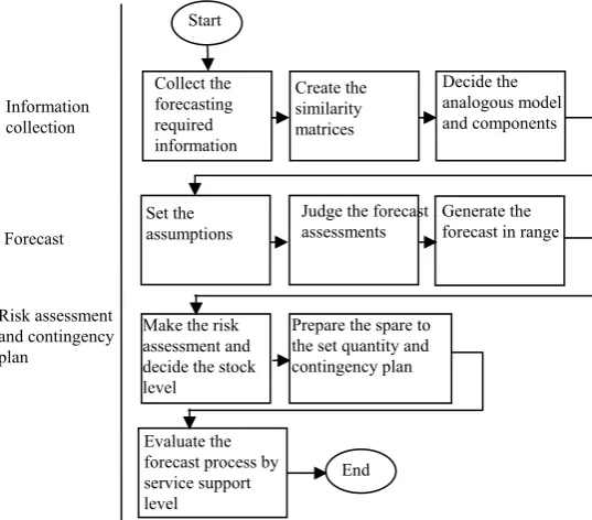
[image:3.595.302.571.416.652.2]Fig. 1 shows the process flow for forecasting ongoing launch product provision buffers. The process starts with the collection of related information and ends with process performance measurement. The process includes four sub-processes; information collection, forecasting mechanism, forecasting execution, measurement and feedback. The detail discussions of each process list in the following subsections.
Fig. 1. The forecasting ongoing launch product provision buffer flow
C. Information Collection
The first step of performing the forecast is to collect information. This information applies for later processes such as building the similarity metrics for deciding the analogous device or as a component base for further forecasting processes. The necessary information lists below [12]:
production specification sales volume
Start
Collect the forecasting required information
Create the similarity matrices
Decide the analogous model and components
Set the assumptions
Judge the forecast assessments
Generate the forecast in range
Make the risk assessment and decide the stock level
Prepare the spare to the set quantity and contingency plan
Evaluate the forecast process by service support level
End Information
collection
Forecast
quality event
spare part acquirement lead time minimum replenishment cycle manufacturing log
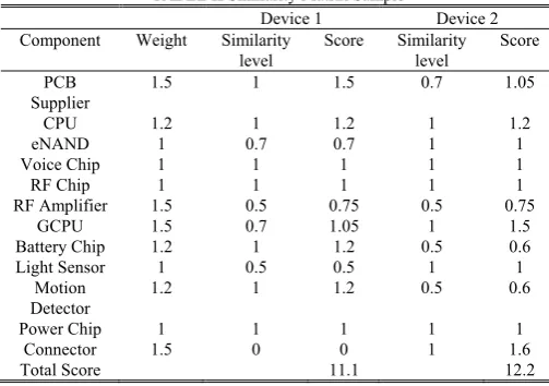
[image:4.595.299.555.60.161.2]From the collected product specifications, the forecaster creates the similarity metrics for reviews and comparison between the analogous product and the chosen product’s data. The results will be then used as the base for the later forecasting process. This study chose smartphone as an example to demonstrate our approach. A similarity matrix sample is provided in Table II. In this table; the similarity level depends on the user’s requirement. The highest level indicates they are the same while, on the contrary, a level of 0 indicates no correlation. The similarity levels are judged by technical staff (from engineering teams and field technicians) by their professional experience. In order to distinguish the difference of the importance of those components, a weight may be added to enhance the verification capability in finding the right analogous product. After all reference products are screened and marked, the analogous product will be chosen, and its historical data will be used in the process.
TABLE II Similarity Matrix Sample
Device 1 Device 2 Component Weight Similarity
level
Score Similarity level
Score
PCB Supplier
1.5 1 1.5 0.7 1.05
CPU 1.2 1 1.2 1 1.2
eNAND 1 0.7 0.7 1 1
Voice Chip 1 1 1 1 1
RF Chip 1 1 1 1 1
RF Amplifier 1.5 0.5 0.75 0.5 0.75
GCPU 1.5 0.7 1.05 1 1.5
Battery Chip 1.2 1 1.2 0.5 0.6
Light Sensor 1 0.5 0.5 1 1
Motion Detector
1.2 1 1.2 0.5 0.6
Power Chip 1 1 1 1 1
Connector 1.5 0 0 1 1.6
Total Score 11.1 12.2
D. The Forecasting
[image:4.595.302.553.188.291.2]Once the analogous product is chosen, this product’s historical data will be used as the forecasting base in calculating the range of the demand for the provision buffer. The method of calculating the spare part buffer shows in Table III. In this formula, there is no argument for sales volume, an annual failure, and provision buffer support period. Extra material change lead time is added to manage the risk of unexpected material change. The extra lead time is due to the possible longest component acquisition lead time multiplied by the possible probability (lead time multiples probability). These four factors are also the assumptions used in the metrics; an example is also provided in Table IV.
TABLE III Forecasting calculation Formula Sales
Volume
Annual Failure Rate
Initial Buffer Support
Material Change
Base Demand
(A)/Usage (AFR)/Week(B) Period/Week(C) Lead Time (D)
=A*B*(C+D)
TABLE IV The pessimistic and optimistic case matrix sample Assumptions Base
Demand
Pessimistic Demand
Optimistic Demand
Chosen Stock Level Sales Volume
1.00
-0.15 0.35 AFR(Annual
Failure Rate)
-0.20 0.20
Material Change (possibility in
week)
0.05 -0.07
Table V The pessimistic and optimistic demand matrix sample Assumptions Base
Demand
Pessimistic Demand
Optimistic Demand
Chosen Stock Level Sales Volume
372.12
304.58 483.75 AFR(Annual
Failure Rate)
297.69 446.54
Material Change (possibility in
week)
389.42 346.15
First, a cross-function committee needs to be formed, and a discussion has to be held. The base values of those four factors are determined and by those factors a base provision buffer level is generated.
After filling the pessimistic and optimistic values in Table IV, and performing the calculation shown in Table III, the forecasting provision buffer range is generated in Table V.
E. Risk Assessment and Contingency Plan
The risk assessment and contingency plan are intertwined, as the cross-function committee manages the risk assessment and product strategy to set the best-balanced provision buffer level. The contingency plan supplements the corresponding plan to meet the possible risk consequences. The evaluation of assessment is based on the overall product strategy, so the assessment needed to be decided by cross-function committee and is not purely the service department’s decision.
Because the stock level sets between pessimistic and optimistic values, the chosen buffer level does not guarantee the stock level fully satisfying the demand. Scenarios may happen where the provision buffer may be overstocked or short, resulting in high costs or customers' dissatisfactory. The contingency plan is not used to prevent such a situation from happening. However, the plan offering a process to mitigate quickly or recover the situation to restore the targeted operation cost and regain customer confidence.
F. Measurement
The purpose of the spare part forecasting final objective is to fulfill the set service level for all scenarios. Adhering to this principle, an evaluation of the forecasting should cover the whole process not just focus on one single point such as accuracy of the forecast or inventory cost.
[image:4.595.41.293.353.530.2] [image:4.595.34.305.728.779.2]The effectiveness of the overall contingency plan to quickly recover the shortages or cope with an overstock is the key point for the process.
V. CONCLUSION
This study discussed the differences between forecasting demand of spare parts for existing products and ongoing launch products. In addition, this study develops a solution approach for forecasting spare part provision buffer for ongoing launch products. This method applies judgment forecasting with assumption-based techniques to overcome the existing hard-to-solve problem of lacking historical data in forecasting ongoing launch product spare part provision buffer.
This approach focuses on an overall performance measurement in forecasting and emphasizes the contingency plan effectiveness in responding to the possible demanding fluctuation. The approach is not perfect and still needs improvements. It does offer an approach to support the product spare part support particularly during the launch period.
REFERENCES
[1] A. Pinder Jr., “After the deal is sealed: Should Sales care about service?”, Aberdeen Group, 2014
[2] “Fixing-First Time Fix: Repair Field Service Efficiency to Enhance
Customer Return”,
http://www.ptc.com/File%20Library/Solutions/All%20Solutions/Aber deen_Fixing_First_Time_Fix_2013.pdf
[3] A. A. Ghobbar and C. H. Friend, “Evaluation of forecasting methods for intermittent parts demand in the field of aviation: a predictive model”, Computers & Operations Research, 30, 2003, pp. 2097–2114. [4] A. L. Beautel and S. Minner, “Saftey stock planning under causal demand forecast”, International Journal of Production Economics, 140, 2012, pp. 637-645.
[5] A. Regattieri, M. Gamberi, R. Gamberini, and R.Manzini, “Managing lumpy demand for aircraft spare parts,” Journal of Air Transport
Management, 11, 2005, pp. 426–431.
[6] D. Apgar, “Assumption-based metrics: recipe for success”, Strategic finance, 2011.
[7] K. B. Kahn, “An exploratory Investigation of new product forecasting practices”, The Journal of Product Innovation Management, 9, 2002, pp. 133-143.
[8] M.E. Trimp, R. Dekker and R.H. Teunter, “Optimise initial spare parts inventories: an analysis and improvement of an electronic decision tool”, Report Econometric Institute, 2004.
[9] B. E. Tysseland, and Ø. Halskau, “Spare parts inventory - A literature review with focus on initial provision and Obsolescence management”,
Proceedings of 19th Annu. NOFOMA Conference, 2007
[10] F. Pérèsand J. C. Grenouilleau, “Initial Spare Parts Supply of an Orbit System”, Aircraft Engineering and Aerospace Technology, 74-3, 2002, pp. 252-262.
[11] R. J. Hyndman and A. B. Koehler, “Another look at measure of forecast accuracy”, International Journal of Forecasting, 22, 2006, pp.
679-688.
[12] R. Dekker, Ç. Pinçe, R. Zuidwijk, and M. N. Jalil , ” On the use of installed base information for spare parts logistics: a review of ideas and industry practice”, International Journal of Production Economics,
143-2, 2013, pp. 536-545.
[13] W. Y. Lee, P. Goodwin, R. Fildes, K. Nikolopoulos, and M. Lawreance, “Providing support for the use of analogies demand forecasting tasks,”
International Journal of Forecasting, 23, 2007, pp. 377-390.
[14] W. van Duinkerken and S. Brinkkemper. "Customized Assumption Planning in Business Planning", 2006.
[15] G. Neves, M. Diallo, and L. J. Lustosa , “ Initial Electronic Spare Parts Stock and Consumption Forecasting”, Investigação Operacional, 28, 2008, pp. 45-58.
[16] H. Lee, S. G. Kim, H. W. Park, and P. Kang, “Pre-launch new product demand forecasting using the Bass model: A statistical and machine
learning-based approach”, Technological Forecasting & Social
Change, 86, 2014, pp. 49-64.
[17] G. S. Lynn, S. P. Schnaars, and, R. B. Skov, “Survey of New Product Forecasting Practices in Industrial High Technology and low Technology Business”, Industrial Marketing Management, l-28, 1999, pp. 565-571.
[18] P. Goodwin, S. Meeran, and K. Dyussekeneva, “The challenges of pre-launch forecasting of adoption time series for new durable products”, International Journal of Forecasting, 30, 2014, pp.
1082-1097.
[19] M. O’Connor, W. Remus, and K. Griggs, “Does updating judgmental forecasts improve forecast accuracy”, International Journal of
Forecasting, 16, 2000, pp. 101-109.
[20] David Apgar, “Assumption-Based Metrics: Recipe for Success”,
Strategic Finance, 2011.
[21] H. B. Skye and D. Dunham, “Critical assumption planning a practical tool for managing business development risk”, Journal of Business