Modeling and Simulation of Partial Blocks of
Flexible Energy System in MATLAB&Simulink
for Temperature Control of Steam/Air Mixture
Martin Pies, Stepan Ozana, Radovan Hajovsky, and Petr Vojcinak
Abstract—The presented article describes two basic techno-logical blocks of so called Flexible power unit which is located in the grounds of the V´ıtkovice company Ostrava in the Czech Republic. The experimental unit was established to research the use of potential energy in a mixture of dry air and superheated steam, which is called air/steam mixture. Creation of air/steam mixture is carried out by mixer whose mathematical model is described in this article. Connection of the mixer to the surrounding FES technology is carried out by steel pipes whose mathematical model is also described in this article. This article aims to outline the temperature control of air/steam mixture at selected technological blocks of flexible energy system. The control is performed through linearized model of the mixer in operating point, which corresponds to the operating point of mixer in a real energy unit. Mathematical models of mixer and steel pipelines are implemented in S-functions with the aim of easy simulation of these blocks in Simulink.
Index Terms—Heat exchangers, Mathematical models, Com-plex systems, Steam, Temperature control.
I. INTRODUCTION
T
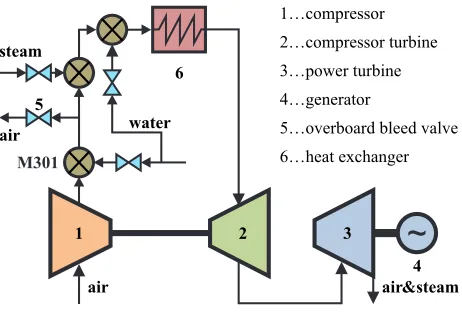
HE paper deals with mathematical model of experimen-tal unit of the power plant with low power, see Fig. 1. The whole mathematical model consists of combination of particular mathematical models of the following technologi-cal components:• superheaters of steam/air mixture
• unheated areas (pipelines)
• mixer
• turbine unit
The mathematical model of experimental power plant is presented. The model serves as a base for simulation of both the power plant dynamics and control principles. The paper describes the scheme of the power plant, the structure of its mathematical model, and software implementation of the model by a computer. Superheaters of steam/air mixture and unheated areas (pipelines) are described by sets of nonlinear partial differential equations and thus represent distributed-parameters systems. Mixers serve for heating/cooling of the mixture or adjustment of the concentration. Their ma-thematical models are based on heat and enthalpy balance equations, and they use XSteam library for Matlab with thermodynamic properties of the media. Turbine unit is composed of compressor, compressor turbine and power turbine.
Manuscript received June 25th, 2013; revised July 25th, 2013. This work
was supported by the project SP2013/168, named “Methods of collecting and transfer of the data in distributed systems” of Student Grant Agency (VSB - Technical University of Ostrava).
[image:1.595.305.536.196.353.2]All authors are with the Department of Cybernetics and Biomedical Engineering, VSB-Technical University of Ostrava, 17. listopadu 2172/15, 70833 Ostrava, Czech Republic, Europe, e-mail: [email protected].
Fig. 1. Simplified model of Flexible Energy System
Dynamics of particular components is modeled by use of Simulink S-functions and FDM (finite difference method) to transfer sets of partial differential equations (PDE) into sets of ordinary differential equations (ODE).
II. MATHEMATICAL MODEL OF HEAT EXCHANGER
Heat exchanger transfers heat energy from a heating media to a heated media. In a typical power plant heat exchanger a tube bundle is located into a gas channel.
The tube bundle transports the heated fluid, the gas channel transports the heating fluid or vice versa. Heat from the heating media is transmitted to the heated media through the walls of the steel tubes. Fig. 2 shows the principal scheme of the physical state variables of a counter-flow heat exchanger. In case of simulation in the designed operating point there are not so rapid changes of pressure and power gas temperature. For this purposes, it is possible to divide the heat exchanger described in [1] into temperature and pressure parts. Temperature part of the heat exchanger is described in Fig. 2.
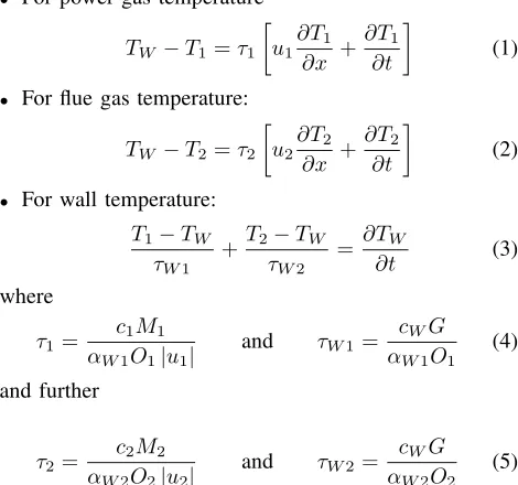
Heat transfer between power gas and the wall of heat ex-changer, and between flue gas and the wall of heat exchanger are described by formulas (1) - (3). Unheated area relates to (1) and modified formula (3) that does not include flue gas temperatureT2.
Fig. 2. Principal scheme of the physical state variables at a counter-flow heat exchanger a) and pipeline b)
• For power gas temperature
TW−T1=τ1
u1 ∂T1
∂x + ∂T1
∂t
(1)
• For flue gas temperature:
TW−T2=τ2
u2 ∂T2
∂x + ∂T2
∂t
(2)
• For wall temperature:
T1−TW
τW1
+T2−TW
τW2
=∂TW
∂t (3)
where
τ1=
c1M1 αW1O1|u1|
and τW1=
cWG
αW1O1 (4)
and further
τ2=
c2M2 αW2O2|u2|
and τW2=
cWG
αW2O2 (5)
It is obvious that temperaturesT1,T2andTW depend both
on time t and distance x. This distance determines current position of the slice in heat exchanger, as shown in Fig. 2.
Pressure effects in the mathematical model of the power plant yet cannot be neglected. Therefore, heat exchanger model is linked to the pressure part which is described by a static linear model of the lumped system. Then power gas pressure in the heat exchangerp1(x, t) can be referred to as power gas temperature at the heat exchanger input p1(MPin, t)and power gas temperature at the heat exchanger outputp1(MPout, t), where MP stands for measuring point. Pressure loss ∆pover the heat exchanger, respectively over unheated area, is calculated from mass flow rate of power gasM1 and pipeline load.
Concentration of the steam w1 in the power gas in the mathematical model of the heat exchanger does not influence the calculation of heat distribution in the heat exchanger. The value of the concentration is copied to the output of the heat exchanger with a delay calculated from the ratio of gas power
TABLE I
HEAT EXCHANGER PARAMETERS symbol description unit c1 heat capacity of power gas [J/kg/K]
c2 heat capacity of flue gas [J/kg/K]
cW heat capacity of superheater’s wall
material
[J/kg/K]
G weight of wall per unit of length in xdirection
[kg/m]
L active length of the wall [m]
M1 power gas mass flow rate [kg/s]
M2 flue gas mass flow rate [kg/s]
O1 surface of wall per unit of length
inxdirection for power gas
[m]
O2 surface of wall per unit of length
inxdirection for flue gas
[m]
u1 velocity of the power gas in x
direction
[m/s]
u2 velocity of the flue gas inx
direc-tion
[m/s]
αW1 heat transfer coefficient between
the wall and the power gas
W/m2/K
αW2 Heat transfer coefficient between
the wall and the flue gas
W/m2/K
[image:2.595.313.539.73.318.2]velocityu1and lengthL. This concentration of the steam in the power gas is then used for further calculations in the injectors and turbine unit.
Fig. 3. Mathematical model of unheated area in Simulink with embedded pressure loss over the pipeline.
[image:2.595.57.292.334.554.2]III. MATHEMATICAL MODEL OF THE MIXER FOR HUMID AIR/WATER
Mathematical model of the mixer for humid air/water, referred to as mixer M301 in Fig. 1 includes algebraic equations describing blending of the water and humid air compressed by a compressor turbine. Mathematical model supposes that the temperature of compressed air coming into mixer M301 is higher than boiling point of the water at a given pressure. Only fulfillment of this condition allows entire evaporation of the water being injected into hot air.
The output of mixerM301is power gas whose composi-tion is determined by concentracomposi-tion of dry air wda and by
concentration of the steamws.
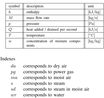
The following table II describes the physical quantities involved in mathematical model of mixerM301.
TABLE II
PHYSICAL QUANTITIES INVOLVED IN MATHEMATICAL MODEL OF MIXER symbol description unit
h enthalpy [kJ/kg]
M mass flow rate [kg/s]
p pressure [Pa]
Q heat added / drained per second [kJ/s]
T temperature [◦C]
w concentration of mixture compo-nents
[kg/kg]
Indexes
da corresponds to dry air pg corresponds to power gas ma corresponds to moist air s corresponds to steam
sd corresponds to steam in moist air wr corresponds to water
The assumption to be fulfilled is that both incoming media have the same pressureppg, corresponding the power
gas pressure at the mixer output. The first step includes determination of water steam concentration ws and dry air
concentration wda in power gas. Quantity of the steam in
power gas is determined by a relative air humiditydin humid air and quantityMwr of the water being evaporated. Ratios
of particular concentrations are illustrated in Fig. 4. Total quantity of power gas is given by formula (6).
Mpg=Mda+Ms (6)
Concentration of humid air coming to the mixerM301, is given by formula (7).
wma=
Mma
Mma+Mwr
(7)
Concentration of the water coming to the mixerM301, is given by formula (8).
wwr=
Mwr
Mma+Mwr
(8)
Humid air includes relative humidity d which must be converted into the form of concentration of the steam in humid air (9).
wsd=
d
[image:3.595.56.272.271.474.2]1 +d (9)
Fig. 4. Definition of power gas in the block representing mixerM301
The concentration of steam in humid airwsd is computed
in previous block compressor. Entire concentration of water steam in power gaswsis computed according (10).
ws= (1−wwr)·wsd+wwr (10)
Concentration of dry air in power gas wda is then a
supplement to one.
wda= 1−ws (11)
Partial pressure of the water steam and a dry air in power gas are determined by (12).
ps=ppg·
1− wda·rda
wda·rda+ws·rs
pda=ppg−ps (12)
whererda andrs are specific gas constants of dry air and
water vapor.
Enthalpy of power gashpg, created as a mixture of humid
air and the water is composed of three enthalpy elements. The first one is the enthalpy of dry air hda. This enthalpy
can be determined by set of the tables stated in [4] using this command:
hda = humde(d,Tma)
d relative humidity level[kg/kg] (d= 0)
Tma temperature of moist air[◦C]
The second element is the enthalpy of water steam hs
contained in a humid air. This enthalpy can be determined by set of the tables stated in [5] using this command:
hs = xsteam(h_pT,psin,Tma)
ps,in partial pressure of the steam in a humid air
[bar](conversionPa→barnecessary) Tma temperature of moist air[◦C]
Forwwr= 0 according (10) we get
ws= (1−0)·wsd+ 0⇒ws=wsd (13)
Then
ps,in=ppg·
1− (1−wsd)·rda (1−wsd)·rda+wsd·rs
=
=ppg·
wsd·rs
(1−wsd)·rda+wsd·rs
pda,in=ppg−ps,in (14)
The third component of the mixture enthalpy is the water enthalpyhwr being injected to the humid air. This enthalpy
can be determined by set of the tables stated in [5] using this command:
hwr = xsteam(’h_pT’,pwr,Twr)
pwr partial pressure of injected water[bar]
Twr temperature of injected water[◦C]
Partial pressure of the water pwr means the difference
of the partial pressures of the water steam before and after mixing. It can be expressed according (15).
pwr=ps−ps,in (15)
Thus it is possible to say that particular enthalpies are functions of the following quantity:
hda=f(Tma), whered= 0
hs=f(Tma, ps,in) hwr=f(Twr, pwr)
(16)
Entire enthalpy of power gas after mixing humid air with the water will be:
hpg=hda·wda+hs·(1−wwr)·wsd+hwr·wwr (17)
In case wwr is zero, then pwr is also zero and relation
(17) turns into:
ws,out= (1−wwr)·wsd+wwr; wwr= 0
ws,out= (1−0)·wsd+ 0; wda,out= 1−wsd
hpg=hda·wda,out+hs·ws,out (18)
In case air at the mixer output M301 does not contain relative humidityd(wsd= 0), thenps,inis zero and relation (17) turns into:
ws,out= (1−wwr)·wsd+wwr; wsd= 0
ws,out= (1−wwr)·0 +wwr; wda,out= 1−wwr
hpg=hda·wda,out+hs·ws,out (19)
Resulting heat of power gas is described by (20).
Qpg =hpg·Mpg (20)
This resulting heat Qpg is one of input parameters for
iterative algorithm described in [6].
IV. TEMPERATURE CONTROL INFES
[image:4.595.304.550.49.203.2]FES unit so far contains 2 control loops. The first one (small, fast) serves for keeping constant temperature TMP6 in measuring point MP6, see Fig. 5. Regulation of the temperature in MP6is carried out by injection M301. The second control loop (big, slow) keeps the constant temper-ature TMP13 at the input of turbine unit MP13. Regulation inMP13is carried out by increasing and decreasing amount
[image:4.595.306.550.240.351.2]Fig. 5. Connection of particular blocks with mathematical models of the components of power plant
Fig. 6. Model for identification of controlled plant in a fast loop
of steam/air mixture behind the compressor, see Fig. 5. The paper deals with the fast loop
Out of the FES unit, for identification of the plant set up in a fast loop out injectionM301and unheated areasPL5 6
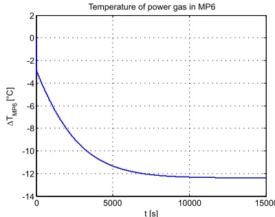
have been chosen, see Fig. 6. Step signal of the water flow was brought to the input of the injection. The step height was 10 %, so the water flow Mwr increased from initial
[image:4.595.323.523.509.667.2]value0.12 kg/sto0.132 kg/s. Temperature response to that change inMP6is shown in Fig. 7.
Fig. 7. Temperature response in MP6to 10 %water flow increase at
M301
The resulting transfer function of the fast loop after identification works out as follows:
G(s) =−1039.1 488.33s+ 1
(2382.1s+ 1) (2.93s+ 1)2 (21)
function (21) a controller has been designed by use ofpidtool
function, resulting in its transfer function (22).
GR(s) =−5·10−
5
−2·10−
4
s (22)
[image:5.595.45.293.79.246.2]Resulting fast loop can be seen in Fig. 8.
Fig. 8. Fast loop in FES
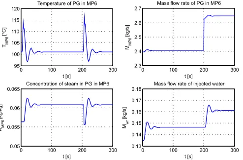
The control loop keeps the temperature of the media in MP6 at TMP6 = 101 ◦C. The loop has been tested with two successive disturbances. The first one represents
10 % increase of air temperature at t = 0 s. The second one, representing 10 % increase of air mass flow, arose at t= 200 s. The resulting responses are shown in Fig. 9.
Fig. 9. Resulting responses in fast loop in FES
V. CONCLUSION
Presented paper was to show possibilities of identification of particular parts of Flexible Energy System unit in order to design a controller. As an example, injection M301
with unheated areasPL5 6have been chosen. Mathematical models of these parts have been introduced at the beginning of the paper.
Implementation of these blocks is carried out by level-2 Simulink S-functions, introduced in [1], [7], [8], [6]. Similar approach use for the fast loop might be used to design a controller for the slow loop. As it is shown in Fig. 5, FES unit contains 4 actuators determined for regulation, three of them are injections and one is a safety valve determined for fast intervention when regulating temperature at turbine input (measuring pointMP13).
REFERENCES
[1] P. Nevriva and L. Vilimec, “Simulation of the power plant dynamics,” in
International Conference on Modeling, Simulation and Control, Cairo, Egypt, 2010.
[2] B. Hanus, M. Olehla, and O. Modrlak,Cislicova regulace technolog-ickych procesu. Brno, Czech Republic: VUTIUM, 2000.
[3] A. P. S. Selvadurai, Partial Differential Equations in Mechanics: Fundamentals, Laplace’s equation, diffusion equation, wave equation. Springer-Verlag, 2000.
[4] D. o. C. Rice University and B. Engineering, “Chbe 301 - material and energy balances,” 2000, [Accessed on 10th Jun 2013]. [Online]. Available: http://www.owlnet.rice.edu/ ceng301/index.html
[5] I. IF-97, “Thermodynamical properties of steam and water,” 1997, [Accessed on 11th Jun 2013]. [Online]. Available: http://www.x-eng.com/
[6] M. Pies, S. Ozana, and Z. Machacek, “Mathematical model of water injected into steam/air mixture determined for temperature control of flexible energy system,” inProceedings of the 10thWSEAS International Conference on SYSTEM SCIENCE and SIMULATION in ENGINEER-ING, W. Press, Ed., Penang, Malaysia, 2011.
[7] P. Nevriva, S. Ozana, M. Pies, and L. Vilimec, “Dynamical model of a power plant superheater,” WSEAS Transactions on Systems, vol. 9, no. 7, pp. 774–783, 2010.
[image:5.595.49.296.348.510.2]