First results from 2+1 dynamical quark flavors on an anisotropic lattice: Light hadron spectroscopy and setting the strange quark mass

First results from

2

þ

1

dynamical quark flavors on an anisotropic lattice: Light-hadron

spectroscopy and setting the strange-quark mass

Huey-Wen Lin,1,*Saul D. Cohen,1Jozef Dudek,1Robert G. Edwards,1Ba´lint Joo´,1David G. Richards,1John Bulava,2 Justin Foley,2Colin Morningstar,2Eric Engelson,3Stephen Wallace,3K. Jimmy Juge,4Nilmani Mathur,5

Michael J. Peardon,6and Sine´ad M. Ryan6

(Hadron Spectrum Collaboration)

1_{Thomas Jefferson National Accelerator Facility, Newport News, Virginia 23606, USA} 2_{Department of Physics, Carnegie Mellon University, Pittsburgh, Pennsylvania 15213, USA}

3_{Department of Physics, University of Maryland, College Park, Maryland 20742, USA} 4_{Department of Physics, University of the Pacific, Stockton, California 95211, USA} 5

Department of Theoretical Physics, Tata Institute of Fundamental Research, Mumbai 400005, India 6_{School of Mathematics, Trinity College, Dublin 2, Ireland}

(Received 24 November 2008; published 3 February 2009)

We present the first light-hadron spectroscopy on a set ofNf¼2þ1dynamical, anisotropic lattices. A convenient set of coordinates that parameterize the two-dimensional plane of light and strange-quark masses is introduced. These coordinates are used to extrapolate data obtained at the simulated values of the quark masses to the physical light and strange-quark point. A measurement of the Sommer scale on these ensembles is made, and the performance of the hybrid Monte Carlo algorithm used for generating the ensembles is estimated.

DOI:10.1103/PhysRevD.79.034502 PACS numbers: 11.15.Ha, 12.38.Gc, 12.38.Lg

I. INTRODUCTION

Understanding the internal structure of nucleons has been a central research topic in nuclear and particle physics for many decades. As detailed experimental data continue to emerge, improved theoretical understanding of the had-ronic spectrum will be needed to learn more about the complex, confining dynamics of quantum chromodynam-ics (QCD). Lattice calculations offer a means of linking experimental data to the Lagrangian of QCD, allowing access to the internal structure of any resonance.

At Jefferson Laboratory (JLab), an ambitious program of research into a range of hadronic excitations is under-way. To date, the Hall B experiment has collected a large amount of data regarding the spectrum of excitations of the nucleons. The Excited Baryon Analysis Center (EBAC) [1,2] aims to review all observed nucleon excitations sys-tematically and to extract reliable parameters describing transitions between resonances and the ground-state nucle-ons. The 12-GeV upgrade of JLab’s CEBAF accelerator will make possible the GlueX experiment, which will produce an unprecedented meson dataset through photo-production. A particular focus will be the spectrum of hadrons with exotic quantum numbers, which can arise when the gluonic field within a meson carries nonvacuum quantum numbers. Such ‘‘hybrid’’ mesons offer a window into the confinement mechanism and will be studied theo-retically in some detail using lattice methods. Lattice

spec-troscopy can determine the properties of isoscalar mesons as well, including any possible candidate glueballs.

Accurate resolution of excited states using lattice QCD has proven difficult. In Euclidean space, excited-state cor-relation functions decay faster than the ground state and at large times are swamped by the larger signals of lower states. To improve the chances of extracting excited states, better temporal resolution of correlation functions is ex-tremely helpful. An anisotropic lattice, where the temporal domain is discretized with a finer grid spacing than its spatial counterpart, is one means of providing this resolu-tion while avoiding the increase in computaresolu-tional cost that would come from reducing the spacing in all directions. This finer resolution must be combined with application of variational techniques to construct operators that overlap predominantly with excited states. In a series of papers [3– 7], techniques to construct operators in irreducible repre-sentations of the cubic group to extract radially and orbi-tally excited states were presented. Application of these techniques to quenched anisotropic lattices shows clear signals as high as the eighth excited state. Also possible on the anisotropic lattice are studies of radiative transitions in meson systems [8] and nucleon-P11 transition form factors [9].

Making the lattice discretization anisotropic comes with a price, however. Since hypercubic symmetry is broken down to just the cubic group, relevant (dimension-four) operators can mix in the lattice action. To ensure the continuum limit of the lattice theory has full Lorentz invariance, a nonperturbative determination of the lattice

action parameters that enforce the symmetry at finite lattice spacing in some low-energy observables has been per-formed [10]. In work to be reported elsewhere, a perturba-tive determination of these action parameters is also being carried out by this collaboration [11].

In this study, we perform three-flavor dynamical calcu-lations with two degenerate light quarks and a strange quark. In a previous study, we tuned a three-flavor lattice action to ensure Lorentz symmetry is restored in appropri-ately chosen low-energy observables. We showed empiri-cally that restoring the symmetry at quark masses below 175 MeV requires only small changes to the action pa-rameters, and no further determinations of these parame-ters is needed within the scope of this study. Our fermion action is a Sheikholeslami-Wohlert discretization, general-ized to the anisotropic lattice [12]. The fermion fields interact with the gluons via three-dimensionally stout-smeared [13] links, and the gluon action is Symanzik improved at the tree level of perturbation theory. To assess the cost of these dynamical calculations, we study the efficiency of the hybrid Monte Carlo (HMC) algorithm in large-scale production simulations.

Using current algorithms and computing resources, it remains impractical to run calculations at the physical value of the light-quark mass. An extrapolation of the light-quark dependence of simulation data is needed. While simulations straddling the correct strange-quark mass have been performed, determining the appropriate choice of mass in the Lagrangian is also problematic;

a priori, this value is not known and changing the bare strange-quark mass affects all lattice observables in a delicate way. This work proposes a simple means of setting the lattice strange-quark mass by examining dimensionless ratios with mild behavior in the light-quark chiral limit. A new set of coordinates, parameterizing the space of theo-ries with different light and strange-quark masses is intro-duced to help this process. We use the ratios

l¼9m2=4m2 and s¼9ð2m2Km2Þ=4m2, inspired by expanding the pseudoscalar meson masses to leading order in chiral perturbation theory.

With this framework in place, the spectrum of some ground-state mesons and baryons is determined and ex-trapolated to the physical quark masses using leading-order chiral perturbation theory. The Sommer scale [14] is de-termined (in units of the Omega-baryon mass) on a subset of our ensembles and extrapolated to the physical quark masses. Using this method, we intend to continue our exploration of excited-state hadrons, including isoscalar and hybrid mesons. A clear means of handling unstable states is needed, and our suite of measurement technology is currently under further development. A study of these techniques on Nf¼2 dynamical lattices gives us

confi-dence that more precise understanding of these states will be forthcoming.

The structure of this paper is as follows: In Sec.II, we will discuss the actions and algorithms used in this work,

and the performance of the method used to generate Monte Carlo ensembles is examined. The details of the measurements we performed on these ensembles is pre-sented in Sec. III. Section IV presents the method we propose to set the strange-quark mass, including the di-mensionless coordinates used for extrapolating quantities measured at unphysical quark masses to the physical the-ory. Our determination of a selection of states in the hadron spectrum and the Sommer scale is given in Sec.V. Some conclusions and future outlook are presented in Sec.VI.

II. SIMULATION DETAILS

In this section details of the lattice action and the per-formance of the hybrid Monte Carlo algorithm are pre-sented. Monte Carlo simulations were performed on lattices with grid spacings of as andatin the spatial and

temporal directions, respectively, and with physical vol-umes L3

sLt, whereLs¼Nsas andLt¼Ntat. Lattices

with extents N3

sNt¼12396, 16396, 163128

and243_{128were employed.}

A. Action

The gauge and fermion actions used in this work are described in great detail in our previous work [10]. For completeness in this paper, we briefly review the essential definitions. For more detailed definitions, see Ref. [10].

For the gauge sector, we use a Symanzik-improved action with tree-level tadpole-improved coefficients

S_G½U ¼ Ncg

X x;ss0

₅

6u4

s

_P ss0ðxÞ

1 12u6

s

_R

ss0ðxÞ

þX x;s 2 g ₄

3u2

su2t

_PstðxÞ 1

12u4

su2t

_RstðxÞ

;

(1)

where_W ¼Re Trð1WÞandW ¼P, the plaquette, or

R, the21rectangular Wilson loop (length two in the direction and one in the direction) with fs; s0g 2

fx; y; zg. The parameter g is the bare gauge anisotropy, Nc¼3indicates the number of colors,is related to the

coupling g2 _{through ¼2N}

c=g2, andus and ut are the

spatial and temporal tadpole factors. This action has lead-ing discretization error at Oða4

s; a2t; g2a2sÞand possesses a

positive-definite transfer matrix, since there is no length-two rectangle in time.

In the fermion sector, we adopt the anisotropic clover fermion action [12]

S_F½U;c;c ¼X x

^

cðxÞ 1

~

u_t

~

utm^0þtW^tþ

1

_f X

s sW^s

1 2 ₁ 2 g f þ 1 _{R 1} ~

utu~2s X

s tsF^ts

þ 1 f 1 ~ u3 s X s<s0 ss0F^ss0

^

where_fis the bare fermion anisotropy and_R¼a_s=a_tis the renormalized anisotropy.s;t,standss0(with¼

½; =2) are Dirac matrices. Hats denote dimensionless variables that connect to dimensionful quantities as quark fieldc^ ¼a3s=2c, bare quark massm^0 ¼m0at, gauge field

strength F^¼aaF¼ ImðPðxÞÞ=4 and ‘‘Wilson

operator’’ W^ r^^=2 (with r^¼ar, ^

¼a2). The gauge links in the fermion action are

three-dimensionally stout-link smeared gauge fields with smearing weight¼0:14andn¼2iterations.u~_sandu~_t are the spatial and temporal tadpole factors from smeared fields, respectively.

In our previous work [10], we found at¼1:5, that the tadpole factors are

u_s¼0:7336; u_t¼1; u~_s¼0:9267;u~_t¼1: (3)

Tuning the anisotropy for all quark masses (even below the chiral limit) gives the desired_g;f

_g¼4:3; _f¼3:4: (4)

B. Algorithm

We use the rational hybrid Monte Carlo (RHMC) algo-rithm for gauge generation [15]. The theoretical aspects of our procedure were discussed in detail in Ref. [10]. Here, we discuss only the aspects that are specific to the calcu-lations presented in this work.

We use rational approximations for both the light-quark fields and for the strange quarks—one field for each light-quark flavor and another one for the strange. We employ even-odd preconditioning for the Wilson clover operator, obtaining the Hamiltonian

H¼1

2 X

x;

Try2X

x

Tr logAeeðmlÞ

X

x

Tr logAeeðmsÞ þSFðmlÞ þSFðmlÞ

þSFðmsÞ SsGStG; (5)

where are the momenta conjugate to the gauge fields; terms involvingA_ee contribute effects due to the parts of the preconditioned clover determinant coming from the submatrix connecting even sites;Ss

G andStG are the parts

of the gauge action involving loops in the spatial directions only and with loops including time direction, respectively; and SFðmlÞ and SFðmsÞ are pseudofermion terms for the

rational approximations to the fermion action correspond-ing to the light- and strange-quark fields, respectively, which we discuss below.

The pseudofermion termsS_FðmÞemploy a rational ap-proximation to the fermion determinant of the even-odd preconditioned clover operator coming from the submatrix connecting the odd sites for a quark with mass m. This submatrix is

Mðm; ~UÞ ¼Aooðm; ~UÞ DoeðU~ÞAee1ðm; ~UÞDeoðU~Þ; (6)

whereAoois the clover operator on the odd sites,Aee1is the

inverse clover operator on the even sites, andD_oeðD_eoÞis the Wilson hopping term connecting odd sites with even (even sites with odd). In all the expressions, U~ denotes stout-smeared gauge fields U, which were smeared as described in Sec.II A.

To construct our pseudofermion actions, we use the rational approximation Ra=bðMyMÞ in partial-fraction form:

Ra=bðMyMÞ ¼ X i

piðMyMþqiÞ1 ðMyMÞa=b; (7)

where we drop the quark-mass dependence ofMfor clarity. The coefficients ,p_i, andq_idefine the approximation and are determined via the Remez algorithm [16,17] applied over the spectral bounds of the operatorMyM. In particu-lar, we needed to compute approximations with ða; bÞ ¼

ð1;4Þ for evaluating the actions (see below), ða; bÞ ¼

ð1;4Þfor pseudofermion refreshment andða; bÞ ¼ ð1;2Þ for our molecular dynamics (MD). Our approximation bounds for the action are shown in TableI. We solve the linear system resulting from applying Ra=b _to

pseudofer-mion fields using the multishift conjugate gradient algo-rithm [18]. We use a stopping relative residuumr <108 in our energy calculations, where the residuum for poleiis

r_i¼jj ðM y

MþqiÞcijj

jjjj ; (8)

whereis the pseudofermion field andc_iis the solution corresponding to the i-th pole. However, since the multi-shift algorithm cannot be restarted, our stopping was based on estimates of ri accumulated with the short-term

recur-rence in the solver algorithm, which may be slightly differ-ent from the true residual as defined in Eq. (8) due to solver stagnation and rounding effects. To minimize rounding effects we accumulated sums and inner products using double precision.

TABLE I. Details of the approximations used for the pseudofermionic actionRð1=4Þ_{. We show the bounds, the number of poles, and}

the maximum error for the approximation to the light and strange pseudofermion terms.

V Light quark Strange quark

atml Bounds No. poles Max. error atms Bounds No. poles Max. error

243_{128 0:0840 (510}6_{, 10) 16 1:810}8 _{0:0743 (10}4_{, 10) 12 8:810}8

Our pseudofermion action terms are

S_F ¼XyX; X¼Rð1=4Þ_ðMy_MÞ¼ X

i

p_ic_i; (9)

individually for each flavor. We do not need to employ multiple pseudofermion fields per flavor in this study.

During our simulation, we adjusted our approximation range by measuring eigenvalue bounds every five trajecto-ries during the process of thermalization. Thereafter, we continued to measure the bounds to ensure we do not suffer from boundary violations.

Our molecular dynamics process employs a rational force

F¼ X

i picy_i

_dMy

dU MþM ydM

dU

ci; (10)

whereiruns over the number of poles in the approximation

Rð1=2Þ_{. Time derivatives are evaluated over the stouted} gauge fieldU~, and only the final sum is recursed down to compute the force for the thin linksU.

We employ a multiple-timescale integration scheme for the molecular dynamics evolution [19] by nesting a second-order Omelyan [20,21] integration step at each timescale. Our largest forces come from the temporal directions: the gauge force fromSt

Gand the temporal forces

generated by the pseudofermions. To mitigate the numeri-cal effort needed [22], we place theSt

Gterm in the action on

a finer timescale than the other terms, and to deal with the temporal forces from the pseudofermion terms, employ an anisotropic timestep with temporal timestepdtof length

dt_t¼dt_s=_MD; (11)

whereMD¼3:5. Apart from the above, we find the forces from Ss

G and the spatial forces from the SF terms to be

within a factor of 2 of each other, so we place them on the same timescale. The forces from the Tr logA_ee terms are

very small in comparison but have small numerical cost, so we place them on the same timescale asSs_GandSF.

We note that the Hamiltonian for the MD does not need to be known as accurately as the one for the energy calculations; all that is required is for the MD to be reversible, area-preserving, and (as a practical matter) for the acceptance rate to be reasonable. To save on numerical effort we solved our systems of linear equations only to a residuumrMDof at mostrMD<106. Correspondingly, we never required the rational approximation to Rð1=2Þ to have a maximum error better than 106, resulting in a smaller number of poles in the approximation than we need for the energy calculations. Further, to make the MD even less numerically intensive, we follow Refs. [23,24] by relaxing the requirements on the residua for individual poles in Rð1=2Þ_{. We use a range ofr}

MD< 104 _{for the smallest shifts andr}

MD<106 for the larger shifts. We tune our molecular dynamics to attain an overall acceptance rate close to 70%. We show in Table II the bounds of the MD rational approximation used for the run with V¼243128, ðatml;atmsÞ ¼ ð0:0840;0:0743Þ.

We show the residua requested in the MD evolution in Table III, and the timesteps and the resulting acceptance rate in TableIV.

C. Thermalization and autocorrelation

During the first segment of each gauge ensemble gen-eration, some special conditions apply. We do not apply the acceptance test during the first Oð10Þtrajectories in each series, which allows a fast initial approach to the vicinity of the equilibrium. Such a scheme is particularly important in the case of simulations starting from totally ordered or disordered configurations. Wherever possible, however, we begin the algorithm with an equilibrated configuration from a simulation at nearby parameters. Also, during this phase (as mentioned above), the minimum and maximum eigenvalue bounds are updated every 5 trajectories.

TABLE II. Details of the approximations used for the forceRð1=2Þ_{. We show the bounds, the number of poles, and the maximum}

error for the approximation to the light and strange pseudofermion terms.

V Light quark Strange quark

atml Bounds No. poles Max. error atms Bounds No. poles Max. error

243_{128 0:0840 (510}6_{, 10) 12 2:510}6 _{0:0743 10}4_{, 10) 10 2:010}6

TABLE III. Requested residua for the poles in the MD force approximation from the smallest shifts (leftmost) to larger shifts (rightmost).

V ðatml; atmsÞ Poles foratml Residua Poles foratms Residua

243_{128 (0:0840,0:0743) 12 10}4_,104_,5105_,5105_, 5105_,105_,105_,

5106_,5106_, 5106_,3106_,106

10 104_,104_,5105_,105_, 105_,105_,5106_,5106_,

Figure1shows its plaquette history for243₁₂₈ vol-ume and atml¼ 0:0840. Both plaquette histories (one

excluding temporal links and the other including only plaquettes with temporal links) show that equilibrium is reached long before 1000 RHMC trajectories. Therefore, to allow for thermalization of our gauge ensembles during the RHMC, we discard the initial 1000 trajectories from each set.

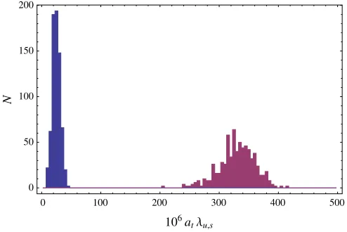
Figure2shows a histogram of the lowest eigenvalues of the Dirac operator MyMfor the light and strange quarks from the ensemble with 243_{128 volume and a}

tml¼

0:0840. The lowest eigenvalues remain safely above

the minimum eigenvalue bounds in which our rational approximation is valid. In addition, they show a clear gap away from zero, where the stability of the algorithm might be compromised.

The autocorrelation function is defined as

ðtÞ ¼ hðOðt0Þ hOiÞðOðt0þtÞ hOiÞi; (12)

whereh. . .imeans taking an average over the samples,tis the trajectory difference in the autocorrelation (from 1 toN

total trajectories), and differentt0(also indexing trajectory number) are averaged. To calculate the integrated autocor-relation lengthintwith a jackknife-estimated errorbar, we first divide the configurations into blocks of size N_b; we calculate _jðtÞ for the jackknife indexjby ignoring con-tributions when eithertort0þtis located within thej-th block and replacing hOibyhOij, the mean value without

thej-th block. With a jackknife dataset of lengthN=Nb, we

calculate integrated autocorrelation length

_intðt_maxÞ ¼1

2þ 1

ðt¼0Þ X tmax

t¼1

ðtÞ; (13)

using the standard jackknife procedure. The autocorrela-tions of the spatial plaquette from gauge ensemblea_tm_l¼

0:0808, 163_{128 are shown in Fig. 3; the integrated} autocorrelation length for the stout-smeared plaquette is about 30 trajectories, which is around twice as large as the unsmeared ones. The integrated autocorrelation length for lowest light and strange eigenvalues are around 13 and 10 trajectories, respectively, as shown in Fig. 4. Figure 5 shows the case of pion and proton correlators at t¼30 on our largest spectrum measurement (518 configurations)

TABLE IV. The two timescales used in the molecular dynamics integration. The spatial timestep for the coarse scale isdt1

s, and for the finer scale it isdt2

s, which we display as a fraction ofdt1s here. We also show our MD timestep anisotropy. On each scale,dtit¼ dti

s=MD. Finally, we show the average acceptance rate for the molecular dynamics with these step sizes.

V ðatml; atmsÞ dt1s dt2s=dt1s MD Acceptance rate 243_{128 (0:0840,0:0743)} 1

16

1

4 3.5 0.71

FIG. 1 (color online). Temporal (left column) and spatial (right column) plaquette history from the ensemble with243_128volume

andatml¼ 0:0840. The x axis is in units of trajectories.

0 100 200 300 400 500 0

50 100 150 200

FIG. 2 (color online). Histogram of the lowest eigenvalues of the Dirac operator for the light and strange quarks from the ensemble with 243_{128 volume and a}

tml¼ 0:0840. The minimum values of the eigenvalues areat¼6:9106 and

2:0104 _{for the light and strange quarks, respectively.}

FIG. 3 (color online). AutocorrelationðtÞand integrated autocorrelation lengthint(in trajectories) for the unsmeared (above) and

smeared (below) plaquette involving only spatial links from the ensemble with163_{128volume anda}

tml¼ 0:0808.

FIG. 4 (color online). AutocorrelationðtÞand integrated autocorrelation lengthint(in trajectories) for the up/down (above) and

strange (below) quark eigenvalues from the ensemble with163_{128volume anda}

ensemble, a_tm_l¼ 0:0808, 163_{128. The integrated} autocorrelation length is about 30 trajectories.

III. MEASUREMENT TECHNIQUES

In this section, the methods used to determine relevant spectroscopy data on the Monte Carlo ensembles are de-scribed. We have used well-established lattice spectros-copy technology throughout this calculation.

To better access ground-state correlation functions, we use the variational method [25,26]. Consider the general-ized eigenvalue problem

CðtÞv¼ðt; t0ÞCðt0Þv; (14)

wheret₀is chosen as the earliest time at which our model (given below) well describes the correlatorC.C_ijðtÞ is a two-point correlation function, composed from the opera-tors Oi and Oj. The correlation matrix can be

approxi-mated by a sum over the lowestNstates:

C_ijðtÞ ¼X 1

n¼1

z_niz_njeEnðtt0Þ_{; (15)}

XN

n¼1

u_niunjeEnðtt0Þ; (16)

whereE_nis the energy of then-th state, andu_mz_n ¼_mn. We extract the energies from the eigenvalues

_nðt; t₀Þ ¼eEnðtt0Þ_{; (17)}

which are obtained by solving

Cðt0Þ1=2CðtÞCðt0Þ1=2vn¼nðt; t0Þvn: (18)

A. Hadron correlation functions

We perform measurements starting from trajectory 1000 on every 10th trajectory, using the EigCG inverter (devel-oped by A. Stathopoulos et al.in Ref. [27]) to calculate quark propagators (with CG residual set to108). We use four sources on each configuration, where a random source location is selected for the first source, and the remaining three are uniformly shifted by Nx;y;z=2 and Nt=4; this

arrangement should reduce potential autocorrelations be-tween configurations. We bin the data over spans of five measurements.

In this work, we construct a33correlator matrixCij

by using three different Gaussian smearing widths (2

f3:0;5:0;6:5g) on the hadron operators. We extract the ground-state principal correlator and fit the ground-state mass using a cosh form. (We also try an exponential form on the principal correlator, and the fit results are consis-tent.) Thetmin dependences (withtmax50) of the fitted masses are shown in Fig.6for the pion, rho, nucleon, and Delta. The fitted masses are very consistent between vari-ous choices of starting time in the fits.

We use meson interpolating fields of the form qq, which overlap with the physical states listed in Table V; charge conjugationCapplies only to particles with zero net flavor. The estimated mass is

ffiffiffiffiffiffiffiffiffiffiffiffiffiffiffiffiffiffiffiffiffiffiffiffiffiffiffiffiffiffiffiffiffi m2=3þ2m2ss=3

q

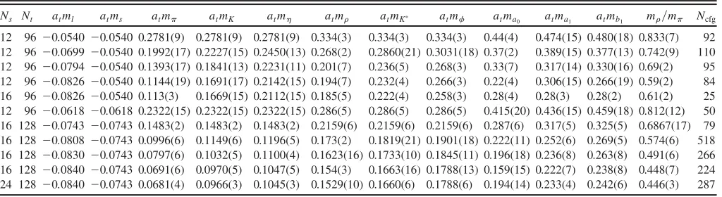
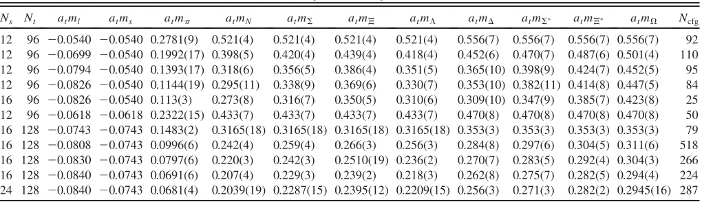
. The ground-state masses are summarized in Table VI. We have two volumes (123 _and163_{) of the lightest ensemble,}

ms¼ 0:0540, and two (163 and 243) on atms¼

0:0743: no major finite-volume effects are observed,

FIG. 5 (color online). AutocorrelationðtÞand integrated autocorrelation lengthint(in trajectories) for the pion (above) and proton

(below) correlator att¼30from the ensemble with163_{128volume anda}

tml¼ 0:0808.

except for thea0mass from theatms¼ 0:0743ensemble

and baryon states fromatms¼ 0:0540.

The octet baryons are calculated using the interpolating field ðq1C45q2Þq1 (with qi¼u=d or s quark); the

uses2ðuC5dÞsþ ðsC5dÞuþ ðuC5sÞd; and the decup-let uses 2ðq2Cð1=2Þð1þ4Þq1Þq1þ ðq1Cð1=2Þ ð1þ4Þq1Þq2 (with ¼xy). The calculated

octet and decuplet ground-state masses are summarized

in Table VII. We observe a finite-volume discrepancy in the baryon sector on the lightest ensemble, atms¼

0:0540. When we extrapolate the hadron masses to the physical limit, we will exclude the small volume sets:123 with atms¼ 0:0540 and 163 with atms¼ 0:0743.

Figures 7and8show the squared-pion-mass dependence of these quantities. We note that for nonstrange hadrons, the sea strange-quark dependences are relatively mild.

At low pion masses, not all the states we calculate on the lattice are safe from decay. To check which particles may decay, we compare the particle masses to the threshold two-particle energies in each channel. The vector mesons could decay to two pseudoscalars in a P wave: ! ðpÞ þðpÞ, K !KðpÞ þðpÞ, and !KðpÞ þ

KðpÞ, where the minimum allowed momentumpon the lattice is 2

Ls. In Fig. 7, we plot the lowest two-particle energy threshold for the ms¼ 0:0540 data with our

two lattice extents (dot-dashed line) and atms¼

0:0743 (dashed). All vector mesons in our calculation are well below threshold. The scalar mesons could decay to

in anSwave, which puts the states slightly below the

FIG. 6 (color online). Pion and rho (above) and proton and Delta (below) fitted masses as functions oftmin, wheretsourcehas been

shifted tot¼0. The bands indicated the final fitted masses summarized in TablesVIandVII.

TABLE V. Meson interpolating operators. States are sorted into columns according to the degree of strangeness from 0 (left two columns) to 1 (right column) and then according to total isospin.

JPC _{I¼1 I¼0 S¼1}

0þ 5 ss K

1 K

0þþ 1 a0

1þþ 5 a1

1þ b1

TABLE VI. Meson masses forNf¼3andNf¼2þ1(in temporal lattice units).

N_s N_t a_tm_l a_tm_s a_tm a_tm_K a_tm a_tm a_tm_K a_tm a_tm_a0 a_tm_a1 a_tm_b1 m=m N_cfg

TABLE VII. Baryon masses forNf¼3andNf¼2þ1(in temporal lattice units).

Ns Nt atml atms atm atmN atm atm atm atm atm atm atm Ncfg

12 96 0:0540 0:0540 0.2781(9) 0.521(4) 0.521(4) 0.521(4) 0.521(4) 0.556(7) 0.556(7) 0.556(7) 0.556(7) 92 12 96 0:0699 0:0540 0.1992(17) 0.398(5) 0.420(4) 0.439(4) 0.418(4) 0.452(6) 0.470(7) 0.487(6) 0.501(4) 110 12 96 0:0794 0:0540 0.1393(17) 0.318(6) 0.356(5) 0.386(4) 0.351(5) 0.365(10) 0.398(9) 0.424(7) 0.452(5) 95 12 96 0:0826 0:0540 0.1144(19) 0.295(11) 0.338(9) 0.369(6) 0.330(7) 0.353(10) 0.382(11) 0.414(8) 0.447(5) 84 16 96 0:0826 0:0540 0.113(3) 0.273(8) 0.316(7) 0.350(5) 0.310(6) 0.309(10) 0.347(9) 0.385(7) 0.423(8) 25 12 96 0:0618 0:0618 0.2322(15) 0.433(7) 0.433(7) 0.433(7) 0.433(7) 0.470(8) 0.470(8) 0.470(8) 0.470(8) 50 16 128 0:0743 0:0743 0.1483(2) 0.3165(18) 0.3165(18) 0.3165(18) 0.3165(18) 0.353(3) 0.353(3) 0.353(3) 0.353(3) 79 16 128 0:0808 0:0743 0.0996(6) 0.242(4) 0.259(4) 0.266(3) 0.256(3) 0.284(8) 0.297(6) 0.304(5) 0.311(6) 518 16 128 0:0830 0:0743 0.0797(6) 0.220(3) 0.242(3) 0.2510(19) 0.236(2) 0.270(7) 0.283(5) 0.292(4) 0.304(3) 266 16 128 0:0840 0:0743 0.0691(6) 0.207(4) 0.229(3) 0.239(2) 0.218(3) 0.262(8) 0.275(7) 0.282(5) 0.294(4) 224 24 128 0:0840 0:0743 0.0681(4) 0.2039(19) 0.2287(15) 0.2395(12) 0.2209(15) 0.256(3) 0.271(3) 0.282(2) 0.2945(16) 287

FIG. 7 (color online). All measured meson masses as functions of the squared pseudoscalar masses. The diamonds and squares are measured withms¼ 0:0540but with two different volumes,12396and16396; the upward-pointing triangles are those with ms¼ 0:0618 and12396 volume; the downward triangles and pentagons are measured withms¼ 0:0743and two different volumes,163_128and243_{128. The (red) dotted-dashed lines indicate the decay thresholds for the12}3_{(upper) and16}3 _(lower)

ms¼ 0:0540ensembles, while the (blue) dashed lines are for the163 (upper) and243(lower)ms¼ 0:0743. The lowest decay thresholds are !ðpÞ þðpÞ,K!KðpÞ þðpÞ,!KðpÞ þKðpÞ,a0!ð0Þ þð0Þ,a1!ð0Þ þð0Þ, and b1!

ð0Þ þ!ð0Þ(with!approximated by), where the minimum allowed momentumpon the lattice is2 Ls.

threshold. Similarly for thea₁andb₁mesonsa₁!ð0Þ þ

ð0Þandb₁ !ð0Þ þ!ð0Þ. In this case, we approximate the!by the, since their masses are similar. Thea₀,a₁, and b₁ (especially for the m_s¼ 0:0743 ensemble) are slightly below the decay threshold. Fortunately, we have two volumes on the lightestmlset; if these states are not

single particle, the ratios of their overlap factors between the two volumes would be of order 2 or higher [28]. We find the ratios (using point-point correlators) to be 0.87 (12), 0.97(6), and 1.01(6), which indicates that our mea-surements are of single-particle states. The decuplet bary-ons are free from decays into an octet baryon. The lowest decay modes are !NðpÞ þðpÞ, !ðpÞ þ ðpÞ, !ðpÞ þðpÞ, as shown in Fig. 8.

Overall, most of the particles are stable. Finally, we measure the renormalized fermion anisot-ropy on the N_f¼2þ1 lattices. We tuned the fermion anisotropy in the three-flavor calculation in Ref. [10],

FIG. 8 (color online). All measured baryon masses as functions of the squared pseudoscalar masses. The diamonds and squares are measured withms¼ 0:0540but with two different volumes,12396and16396; the upward-pointing triangles are those with ms¼ 0:0618 and12396 volume; the downward triangles and pentagons are measured withms¼ 0:0743and two different volumes,163_128and243_{128. The (red) dotted-dashed lines indicate the decay thresholds for the12}3_{(upper) and16}3 _(lower)

ms¼ 0:0540ensembles, while the (blue) dashed lines are for the163 (upper) and243(lower)ms¼ 0:0743. The lowest decay thresholds are!NðpÞ þðpÞ,!ðpÞ þðpÞ,!ðpÞ þðpÞ, where the minimum allowed momentumpon the lattice is2

Ls.

TABLE VIII. Sommer scaler0=as.

Ns Nt atml atms r0=as

where we found that the fermion action coefficients are consistent for bare PCAC quark masses up to about 175 MeV. Figure 9 shows the meson dispersion on the 243_128,a

tml¼ 0:0840andatms¼ 0:0743

ensem-bles. The effective mass plots are shown for the ground-state principal correlators at momentap¼2

Lsnwithn2

f0;1;2;3g; the fitted range and extracted energies are shown as straight lines across the effective mass plots. The inset shows the fitted renormalized fermion anisotropy at each n2_{. The speed of light c is measured from the} energy of the boosted hadron using a2

tEHðpÞ2 ¼

a2

tEHð0Þ2þc 2

2

R 42

N2

s n

2_{. The values ofc from the pion and}

rho mesons are about 2 and 3 standard deviations away from unity. Such a small deviation is also expected on isotropic lattices. For example,cfor the pion and rho are about 2 standard deviations away from unity on the MILC coarse asqtad lattice ensembles [29].

B. Static-quark potential

VðrÞ, the energy of two static color sources separated by distance rprovides a useful reference scale for spectrum calculations. This is most usefully described by the Sommer parameterr₀, defined by the condition

r2@VðrÞ

@r r¼r0

¼1:65: (19)

The potential is computed by measuring correlations between operators creating a static color source in the fundamental representation of SU(3), connected via a gauge covariant parallel tranporter to a source in the 3 representation. The gauge connector can be formed by any sum of path-ordered products of link variables that respects the symmetry of rotations about the inter-source axis. Better ground-state operators are formed by using stout-smeared link variables in the path-ordered

connec-FIG. 9 (color online). Effective-mass plots using the ground-state principal correlators from the pion and rho-meson masses at four different momenta on the lightest ensemble (ms¼ 0:0743) with volume243128. The insets show the energy squared in temporal lattice units versusn2_{, which is related to the momentum byp}2_¼42

L2

s n

2_.

0 10 20 30 40 50

t/at

0.1 0.2 0.3 0.4 0.5 0.6

at Veff

(r)

r/a_s=1 r/a

s=2

r/a

s=3

r/a_s=4 r/a_s=5 r/a_s=6 r/a

s=7

r/a

s=8

1 2 3 4 5 6 7 8

r/as

0.1 0.2 0.3 0.4 0.5

at

V(r)

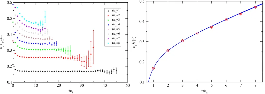
FIG. 10 (color online). Results for the static-quark potential for theatml¼ 0:0808,atms¼ 0:0743mass set. The left panel shows the effective energies,atVeffðrÞfor eachr. The right panel shows the resulting fit to the potential using Eq. (20).

tions and by using an operator optimized using the varia-tional method.

A basis of five operators is constructed from the set of straight connectors and staples linking the midpoint be-tween the two color sources. In forming the temporal correlators, straight, unsmeared temporal links are used for the propagator of the static source. A five-by-five correlation matrix Gijðr; tÞ is then computed for a range

of time separationst and values ofr2 f1; N_x=2galong a lattice axis. As outlined in the previous section, this corre-lation matrix can be analyzed using the variational method to make a more reliable ground-state energy extraction.

Once the potential energy for a range of values ofrhas been determined, the data are compared with the Cornell model

VðrÞ ¼V₀þ

rþr; (20)

and best-fit values for the parameters , and V0 are determined. See an example from one of our ensembles (atml¼ 0:0808andatms¼ 0:0743) in Fig.10. In all

cases, a small range ofrvalues that spanr0are used. Once values of these parameters are computed, a value ofr0was derived from Eq. (19). The QCD flux tube is expected to break in the presence of dynamical quarks and the ground state of the system should not be modeled by the Cornell potential at large separations. We fit the data to Eq. (19) in a sufficiently small range ofrsuch that this issue does not arise. No good evidence of this ‘‘string-breaking’’ effect was observed in our data at larger separations. This obser-vation fits with previous investigations [30], which estab-lished the need to include appropriate operators that construct two disconnected static-source–light-quark sys-tems to measure the full spectrum.

IV. CHOOSING THE BARE STRANGE-QUARK MASS

The appropriate value for the strange-quark mass in the lattice action is not knowna priori. The Wilson formula-tion makes the task of choosing a sensible value for this

parameter more difficult, as the breaking of chiral symme-try at the action level induces an additive mass renormal-ization. In dynamical simulations, changes to the strange-quark mass parameter in the action cause all observables to change. We suggest that a helpful starting point for solving this issue is to determine where reference simulations lie in a parameterized two-dimensional coordinate system. Note that to leading order in chiral perturbation theory, the pseudoscalar masses are related to the quark masses via

m2

P¼2Bðmq1þmq2Þ; (21)

where B is a low-energy constant and mqi are the quark masses that compose the meson. The light-quark depen-dence can be eliminated using the linear combination ð2m2

Km2Þ. A useful property of a new coordinate system

would be to remove all explicit dependence on the lattice cutoff. Such a dependence can be suppressed (if not com-pletely removed) by taking ratios of hadron masses. One good candidate is the baryon mass, which is stable against QCD decays and which has a simplified chiral extrapolation due to its lack of light valence quarks. An alternative is the ð1=2Þ, which also decays only weakly and is statistically clean to measure. AppendixAshows a comparison between these two choices. Therefore, we suggest two dimensionless coordinates,lands:

l¼ 9m2

4m2

; (22)

s¼9ð2m

2

Km2Þ

4m2 ; (23)

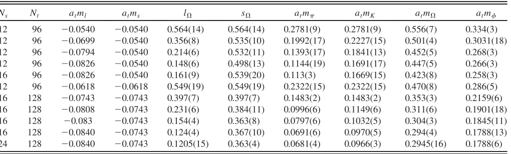
where the factor of 9=4 is a convenient normalization, which makesl ¼s¼1in the static-quark limit. Note that three-flavor-degenerate theories lie on the diagonal line across the unit square. Table IX summarizes all the fl; sg values calculated in this work. Hadron masses are taken from TablesVIandVIIin Sec.V.

In Fig. 11, we locate all the simulations performed in this work using theirlscoordinates. The dashed line

TABLE IX. Values ofl ands.

Ns Nt atml atms l s atm atmK atm atm

runs horizontally from the physical point. We add two more strange-mass candidates 0:0618,0:0743, which are the points on the diagonal line. The choice of0:0743 seems to anchor the correctmsvalue forNf¼3within one

standard deviation of physical. Since we expect only a few percent deviation coming from the next-to-leading effects ons, we settle onatms¼ 0:0743for our final choice of

strange bare mass; the points to the left of the Nf¼3

points are Nf¼2þ1 points with fixed strange input

parameters. At the lightest simulation point,sonly differs fromN_f¼3by less than2. The running of the quantity

sis indeed small and is thus a good means for tuning the strange-quark mass for fixed-simulation. We note how-ever, that the trajectory followed by simulations as bare lattice parameters are changed is dependent on the details of the lattice action and is not universal; different actions may follow different paths as their bare parameters change.

V. EXTRAPOLATION TO THE PHYSICAL QUARK MASSES

Following the discussion in Sec.IV, we adopt the coor-dinatesl ands to perform extrapolation of the meson and baryon masses. To avoid the ambiguity in the lattice-spacing determination, we extrapolate mass ratios atmH

atm

using the simplest ansatz consistent with leading-order chiral effective theory,

_m H m

_n

¼c0þcllþcss; (24)

with n¼2 for pseudoscalar mesons and n¼1 for all other hadrons. With such a parameterization, care is needed to take account of the statistical errors of l and

s in the fit.1Consider a general fit of the formf¼aþ

bxþcy, wheref,x, andyare all quantities with statistical error. We wish to find the combination of a,b,c, which minimizes

X

i

ðfða; b; c;x_i; y_iÞ hf_iiÞ2

2

fiþb 22

xiþc 22

yi

; (25)

where i indexes different data points fx; y; fg, h. . .i indi-cates a mean over all configurations andis the statistical error of each quantity. The extrapolation [minimizing a quantity as in Eq. (25) withf¼mH

m,x¼landy¼s] is

taken to physical fl; sg, and we then takem as experi-mental input to make physical predictions.

A. Hadrons

The2=doffor the fits of hadronic data are all around or smaller than 1 for both meson and baryon masses. Figures 12 and 13 show the ‘‘sliced’’ plots of selected mass ratio with fixed l (or s). The s are almost a constant for the same seaa_tm_s; this is why we see almost a single extrapolated line in the left column of the figures. The hadron masses linearly increase withl and decrease with s. The ratio of m=m is almost constant with respect tos, indicating its insensitivity to the sea strange mass. The strange-mass dependence is almost completely canceled out in such a combination. Later in AppendixA, we see the quantityð2m2

Km2Þ=m2is relatively constant

with respect to changes inm2

.

Figure14and the first column in TableXsummarize all of our extrapolated masses along with the experimental values. The second half of the plots shows the relative discrepancy in percent between our calculation and the experimental numbers. The meson sector appears to have good agreement with experiment; overall, 0.1–4.3% dis-crepancy from experimental values. The biggest discrep-ancy comes in the , which we estimate using a combination of light and strange pesudoscalar mesons. All the vector mesons are in good consistency with experi-ment; themeson is only1:2away. These vector mesons are below the decay threshold on our ensemble; no decays are observed. The extrapolated scalar mesona₀ is consis-tent with the resonance at 980 MeV. The b₁ meson is slightly higher than a1, and both of them are2–3away from experiment.

The baryon sector, on the other hand, does not work as well as the meson extrapolation. Nonstrange baryons, such

FIG. 11 (color online). The location of the dynamical ensem-bles used in this work in thesl plane. The circle (black)

indicates the physical pointflphys ; sphys g. The (red) diamonds and squares are generated on 123_{96 and 16}3_{96 lattices with}

atms¼ 0:0540; the (green) upper triangle is the ensemble on a

123_{96lattice witha}

tms¼ 0:0618and (blue) upside-down triangles and pentagons represent the ensembles on163₁₂₈

and243128lattices withatms¼ 0:0743. Detailed parame-ters can be found in TableIX. The horizontal dashed (pink) line indicates constants from the physical point and the diagonal

line indicates three-flavor degenerate theories.

FIG. 12 (color online). Selected meson mass ratios as functions oflands. Differently shaded (or colored) points correspond to

the atml;s combinations in Fig. 15; detailed numbers can be found in Table VI. The smaller-volume ensemblesfatml; atmsg ¼

f0:0826;0:0540g and f0:0840;0:0743g are excluded from the fits. The lines indicate the ‘‘projected’’ leading chiral extrapolation fit inl ands, while keeping the other one fixed. The black (circular) point is the extrapolated point at physicall

as nucleon and Delta, have the biggest discrepancy, by as much as 8:5. This is likely due to contributions from next-to-leading-order chiral perturbation theory (or

pion-loop contributions), which are not as negligible as the meson ones. This becomes evident as we increase the number of strange quarks in the baryon: the discrepancy

FIG. 13 (color online). Selected baryon mass ratios as functions of thelands. Differently shaded (or colored) points correspond

to theatml;s combinations in Fig.15; detailed numbers can be found in TableVII. The smaller-volume ensemblesfatml; atmsg ¼

f0:0826;0:0540g and f0:0840;0:0743g are excluded from the fits. The lines indicate the ‘‘projected’’ leading chiral extrapolation fit inl ands, while keeping the other one fixed. The black (circular) point is the extrapolated point at physicall

ands.

is smaller in the Sigma and cascade. To have better control of the chiral extrapolation to higher order, we must have better statistics on these measurements; this will be a task for the near future once we complete all of our gauge generation.

Finally, we compare the extrapolation results using all

a_tm_s ensembles and using a single ensemble of either

a_tm_s¼ 0:0540 or a_tm_s¼ 0:0743 alone; results are summarized in TableX. In both cases, themeasurements are in good agreement with experiment; this is expected onceis fixed to 1.672 GeV. However, the kaon masses from theatms¼ 0:0540ensemble are almost 17% away

from experimental ones. This is also not surprising since the atms¼ 0:0540 ensemble was selected using the J

parameter strange-quark mass setting, where MILC had seen a 14–25% discrepancy in the strange-quark mass tuning. The kaon mass from the atms¼ 0:0743

en-semble, on the other hand, is only 3 away from the physical one, which is relatively close for a tuning using

degenerate light and strange masses. The extrapolations using atms¼ 0:0743 alone versus all atms ensembles

are in rough agreement within a few , indicating that

atms¼ 0:0743is a good candidate for gauge generation.

400 500 600 700 800 900 1000 1100 1200 1300 1400 1500 1600

Hadron mass (MeV)

η ρ

K*

ϕ

a 0

a₁ b1

N

Σ Ξ

Λ ∆

Σ*

Ξ*

-12 -10 -8 -6 -4 -2 0 2 4 6 8 10 12

Deviation from experiment (%)

η

ρ _K*

ϕ

a₀

a₁ b₁

N

Σ Ξ

Λ ∆

Σ*

Ξ*

FIG. 14 (color online). Summary of the extrapolated hadron masses compared with their experimental values.

TABLE X. Hadron masses (in GeV) obtained from ðmH=mÞn (n¼2 for pseudoscalar mesons and 1 for the other hadrons)

extrapolations using different sea-strange ensembles. The square brackets indicate the2_{=dof for each fit (withdof¼6), and the}

second parentheses indicate the percent deviation of the central value from experimental values.

all atms¼ 0:0743 atms¼ 0:0540 mK n/a 0.476(6)[0.14](3.74) 0.578(13)[0.17](16.7) mn 0.570(5)[0.04](4.29) 0.546(5)[0.25](0.2) 0.677(12)[0.62](23.79) mp 0.780(8)[0.72](1.27) 0.812(8)[0.12](5.4) 0.64(3)[2.96](16.52) mK 0.896(7)[0.49](0.5) 0.912(7)[0.1](2.27) 0.828(20)[1.7](7.19) m 1.011(6)[0.42](0.84) 1.012(7)[0.15](0.75) 1.007(18)[0.97](1.3) ma0 0.98(6)[0.3](0.13) 0.98(7)[0.11](0.49) 1.06(17)[0.05](7.73)

ma1 1.19(3)[0.7](3.39) 1.23(3)[1.1](0.1) 1.03(7)[0.09](16.17)

mb1 1.26(3)[1.09](2.28) 1.33(4)[0.41](8.47) 1.03(7)[0.53](16.18)

mp 1.020(12)[0.49](8.48) 1.033(13)[0.26](9.87) 0.93(3)[0.43](0.72) m 1.216(10)[0.62](2.15) 1.226(11)[0.98](3.03) 1.16(2)[0.5](2.74)

m 1.319(9)[0.8](0.08) 1.309(11)[0.63](0.69) 1.334(20)[0.62](1.22)

m 1.166(10)[1.18](4.51) 1.167(12)[1.57](4.56) 1.13(2)[0.53](1.27)

m 1.325(12)[0.97](7.57) 1.367(15)[0.36](10.93) 1.16(2)[4.81](5.78)

m 1.461(9)[1.07](5.52) 1.491(9)[0.4](7.67) 1.34(2)[2.47](3.06)

m 1.566(6)[1.](2.17) 1.582(5)[0.84](3.16) 1.506(18)[1.81](1.79)

B. Sommer scale at the physical quark masses

Using the static-potential data in Table VIII, we can extrapolater0m to the physical limit usingfl; sg coor-dinates and the simplest functional form

r₀m¼f₀þf_llþf_ss: (26)

Once this parameterization is known,mserves as experi-mental input andr₀becomes a physical prediction. Using this technique, we determine the Sommer scale in the physical limit, rphys₀ . We compose a dimensionless ratio

r0

asðatmÞ and extrapolate using Eq. (25). After a chiral extrapolation including all three strange ensembles, we find the dimensionless ratio r₀m=_R¼1:100ð11Þ. The ‘‘sliced’’ fits projected on to a single parameter l (left) ands(right) at each point are shown in Fig.16. Then we substitute in the physical Omega mass to find

rphys₀ ¼0:454ð5Þ fm; (27)

with2=dof ¼1:5ð0:7Þanddof¼6. The biggest2 con-tribution comes from theatms¼ 0:0618ensemble. If we

drop it, we improve 2_{=dof to 0.92(0.60) but find only a} small change torphys₀ ¼0:451ð5Þ fm. Extrapolating using a ratio with m rather than m givesr

phys

0 ¼0:446ð4Þfm. These data are consistent with the MILC result in Ref. [32], which gave a continuum-extrapolated value of 0.462 (12) fm.

C. Scale setting

We determined the lattice cutoff (in physical units) at the physical point. Again, we follow the strategy of using the Omega-baryon to set the scale in physical units. A best fit of all simulation data to the model

a_tm ¼d₀þd_llþd_ss (28)

has 2=dof¼3:10. Inputting the physical coordinates fl; sg ¼ f0:0153;0:379g yields at¼0:035 06ð23Þfm

and a_s¼0:1227ð8Þfm.2 The low quality of the fit pro-vides us with further incentive to avoid expressing the lattice cutoff scale in physical units except in an extrapo-lation to the continuum. No continuum extrapoextrapo-lation is possible with our current data set, since all our ensembles have a common value of the gauge coupling.

VI. CONCLUSION AND OUTLOOK

This paper presents our first investigation of a number of states in the light hadron spectrum of QCD with N_f¼

2þ1 dynamical flavors. Simulations were performed on anisotropic lattices with the ratio of spatial and temporal scales fixed nonperturbatively toas=at¼3:5.

The focus of this work has been to test a simple method for determining the bare strange-quark mass, to allow us to approach the physical theory. Conventionally, this has been difficult to achieve, as there is delicate coupling between lattice action parameters and the cutoff scale. We found it extremely useful to introduce a pair of coordinates,sand

l to parameterize the two-dimensional space of quark mass values. The degenerate three-flavor theory corre-sponds to the linel ¼s. To leading order in the chiral effective theory, these two coordinates are proportional to the strange- and light-quark masses. These coordinates have been shown to be useful for our simulations since

s shows mild dependence on changes to the lattice light-quark mass. This shows that a good approximate value of the strange quark mass can be found by following the three-flavor degenerate line to the point where s takes its physical value before changing the light-quark masses, a strategy adopted in this calculation.

With a lattice strange-quark mass close to the physical value, a number of the simplest light hadrons were inves-tigated. The finite-volume effects for the mesons were checked on our data sets and found to be mild. Of the states we investigated, thea0,a1, andb1mesons could have decayed on our lattices. However, checking the overlap

FIG. 16 (color online). ‘‘Slices’’ ofr0m=Ras functions ofl (left) ands (middle). The straight lines are the fitted functions

according to Eq. (25). The assignment of colors is shown in the Fig.15.

2_{Using the values of a}

t set bym at the physical point, we

estimate the range of pion masses to be 0.62 to 1.52 GeV for the heaviest strange (ms¼ 0:0540) ensembles, 1.3 GeV for the ms¼ 0:0618ones and 0.37 to 0.81 GeV for thems¼ 0:0743 ones.

factors of the interpolating operators with the ground states on different volumes suggests that the states we measured are predominantly resonances. For the octet and decuplet baryons, a similar analysis predicts that the,, and are stable in our study. At the heavy strange-quark masses where calculations on 123 lattices were performed, some finite-volume effects were seen, but they were negligible on the larger lattice volumes.

Physical predictions have been made by extrapolating simulation data as a function of these coordinates to the physical point,fl; sg ¼ f0:0153;0:379g. These extrapo-lations have been seen to be robust and have the advantage of making no reference to the lattice cutoff. This should enable reliable contact with chiral effective theories to be made. In this analysis, only the most naive extrapolations have been performed, and some discrepancy between ex-trapolated hadron masses and experimental data remains. It is encouraging to note that at worst, this discrepancy is less than 5% for mesons. The largest mismatch occurs in the nucleon-mass determination, which disagrees with experi-ment by 8%. It is very likely that the use of a naive extrapolation is responsible. No extrapolation to the con-tinuum limit has been carried out; at present, calculations at a single value of the gauge coupling have been performed, so no such analysis is possible.

The collaboration has begun to explore more challeng-ing measurements on the ensembles described in this work. The anisotropic lattice should allow us to resolve heavier excited states and those states that have traditionally been statistically rather imprecise with better accuracy. These more difficult calculations include the hybrid and isoscalar mesons, including the glueballs. We are confident that a detailed picture of a broad range of light-hadron physics will emerge soon from these analyses.

ACKNOWLEDGMENTS

This work was done using theCHROMA software suite [33] on clusters at Jefferson Laboratory using time awarded under the USQCD Initiative. We thank Andreas Stathopoulos and Kostas Orginos for implementing the EigCG inverter [27] in theCHROMAlibrary, which greatly sped up our calculations. This research used the resources of the National Center for Computational Sciences at Oak Ridge National Laboratory, which is supported by the Office of Science of the Department of Energy under Contract No. DE-AC05-00OR22725. In particular, we made use of the Jaguar Cray XT facility, using time allo-cated through the U.S. DOE INCITE program. This re-search was supported in part by the National Science Foundation under Contract Nos. NSF-PHY-0653315 and NSF-PHY-0510020 through TeraGrid resources provided by Pittsburgh Supercomputing Center (PSC), San Diego Supercomputing Center (SDSC), and the Texas Advanced Computing Center (TACC). In particular, we made use of the BigBen Cray XT3 system at PSC, the BlueGene/L

system at SDSC, and the Ranger Infiniband Constellation Cluster at TACC. J. B., J. F. and C. M. were supported by Grant Nos. NSF-PHY-0653315 and NSF-PHY-0510020; E. E. and S. W. were supported by DOE Grant No. DE-FG02-93ER-40762; N. M. was supported under Grant No. DST-SR/S2/RJN-19/2007. M. P. and S. R. were sup-ported by the Science Foundation Ireland under research Grant Nos. 04/BRG/P0275, 04/BRG/P0266, 06/RFP/ PHY061, and 07/RFP/PHYF168. M. P. and S. R. are ex-tremely grateful for the generous hospitality of the theory center at TJNAF while this research was carried out. This work was supported by DOE Contract No. DE-AC05-06OR23177, under which Jefferson Science Associates, LLC, operates Jefferson Laboratory. The U.S. Government retains a nonexclusive, paid-up, irrevocable, world-wide license to publish or reproduce this manuscript for U.S. Government purposes.

APPENDIX A: ALTERNATIVE POSSIBILITIES FORfl; sg_X

In this work, we have been using the dimensionless parametersfl; sg [defined in Eq. (22)] to set the strange-quark mass and to extrapolate hadron mass ratios. In this section, we discuss alternatives to the : 1). the strange vector meson, which like thecontains no valence up or down quarks; 2). the octet , which is statistically cleaner to measure than the decuplet; 3). a linear combi-nation of octet baryons,2, where the linear combi-nation is selected to hopefully cancel out the leading-order up/down-quark dependence.

We first look at the sX dependence on the sea strange

mass, a similar strategy as described in Sec.IV. Figure17is a similar to Fig.11, which we used to tune the sea strange quarks. The blue upside-down triangles (V¼163_{) and} pentagon (243_{) are points from the a}

tms¼ 0:0743

en-sembles, the red diamonds (V¼123_{) and squares (16}3_{) are} from atms¼ 0:0540 and the green triangles are from atms¼ 0:0618. The leftmost plot corresponds to X¼ , and it shows the strong dependence ofsX onatmsthat

we are looking for to tune the strange-quark mass. TheX¼ could be an alternative for setting the strange quark mass. This result also agrees with our choice of sea strange at a_tm_s¼ 0:0743. The results from s (middle plot) show negligible sea strange dependence on Nf ¼2þ1;

this makes it a poor index for tuning the bare strange quark, since we cannot distinguish when sea quarks are not de-generate anymore. Somehow the remaining freedom of the light quark in thebaryon dominates the chiral behavior, since the a_tm_s¼ 0:0743 set is running up toward the physical line. This running is greatly improved when we considerX¼2, which lies on the physical line for alllX. However, it is a poor candidate for tuning, since it

shows little dependence onsX.

accord-ing to the minimization process described in Eq. (25)] uses all threea_tm_sensembles without the smaller volume on the lightest ensemble of a_tm_s¼ 0:0540 and a_tm_s¼

0:0743 sets. The X¼2 has the poorest 2=dof among them all; we will throw it away for reliable extrapo-lation comparison. TheX¼fits have similar2_=dofto the but slightly worse. This is possibly due to its in-sensitivity to s during the extrapolation. The X¼

should be quantitatively comparable to X¼ coordi-nates. However, due to the lightness of the mass, it is not difficult to see that the next-leading-order contributions to the extrapolation form would be larger than theX¼, causing it to be a slightly poorer fit at leading order. Even though the fit usingX¼ has a smaller statistical error, we expect the systematic error to be higher thanX¼.

We will leave estimation of the systematics to future precision calculations where statistical error will be more reasonable. Still, we see good consistency betweenX ¼

and X¼ results, which reinforces our belief in the stability of extrapolations using the dimensionless coordi-natesfl; sg.

APPENDIX B: STRANGE-SETTING COMPARISONS

The J parameter [34] is one common way to set the strange-quark mass; it is defined as

J¼dmV dmP

¼mKðmmÞ

2ðm2

Km2Þ

: (B1)

TABLE XI. Hadron masses (in GeV) obtained from ðmH=mXÞn (n¼2 for pseudoscalar mesons and 1 for the other hadrons) extrapolations in terms offl; sgX with X2 f; ;;2g using all sea-strange ensembles. The square brackets indicate the 2_{=dofon the fit and the second parentheses denote the central value deviations from experimental values in percent.}

X¼ X¼ X¼ X¼2

atm 0.570(5)[0.04](4.29) 0.569(2)[0.14](4.04) 0.570(3)[0.1](4.2) 0.569(3)[0.11](4.1) atm 0.780(8)[0.72](1.27) 0.795(5)[2.08](3.21) 0.785(7)[2.44](1.93) 0.819(7)[3.95](6.31) atmK 0.896(7)[0.49](0.5) 0.907(3)[1.77](1.69) 0.905(5)[2.3](1.42) 0.933(5)[3.73](4.55) atm 1.011(6)[0.42](0.84) n/a 1.023(5)[1.92](0.32) 1.044(5)[3.](2.32) atma0 0.98(6)[0.3](0.13) 0.99(6)[0.29](0.35) 0.97(7)[0.33](1.98) 1.00(7)[0.31](1.6)

atma1 1.19(3)[0.7](3.39) 1.21(3)[0.76](2.02) 1.18(3)[1.42](3.88) 1.23(3)[1.73](0.32)

atmb1 1.26(3)[1.39](2.28) 1.28(3)[1.85](4.06) 1.27(3)[1.9](2.89) 1.32(3)[2.58](7.03)

atmp 1.020(12)[0.49](8.48) 1.029(10)[0.89](9.45) 1.007(6)[0.06](7.09) 1.048(9)[0.63](11.5) atm 1.216(10)[0.62](2.15) 1.226(8)[1.21](3.06) 1.211(4)[2.7](1.75) 1.243(7)[3.81](4.43)

atm 1.319(9)[0.8](0.08) 1.323(7)[1.42](0.39) n/a 1.345(4)[3.47](2.02)

atm 1.166(10)[1.18](4.51) 1.176(8)[1.86](5.38) 1.161(3)[0.54](4.06) 1.194(6)[1.6](6.97)

atm 1.325(12)[0.97](7.57) 1.335(17)[1.38](8.36) 1.312(18)[1.68](6.51) 1.356(19)[2.66](10.07)

atm 1.461(9)[1.07](5.52) 1.464(15)[1.41](5.72) 1.450(15)[1.41](4.66) 1.490(17)[2.49](7.58)

atm 1.566(6)[1.](2.17) 1.568(12)[1.03](2.3) 1.561(13)[1.15](1.8) 1.593(15)[2.22](3.94)

atm n/a 1.685(10)[0.37](0.8) 1.683(12)[0.89](0.64) 1.708(12)[1.82](2.17)

FIG. 17 (color online). ThesXlXplot withX¼(left)(middle) and the linear combination2forNf ¼3andNf¼

2þ1 at ¼1:5. The circle (black) indicates the physical point flphys_X ; sphys_X g. The (red) diamonds and squares are 123_{96 and} 163_96froma

tms¼ 0:0540ensembles; (green) upper triangles are from12396fromatms¼ 0:0618and (blue) upside-down triangles and pentagons are from163_128and243_128froma

tms¼ 0:0743ensembles. Detailed parameters can be found in TableIX. The horizontal dashed (pink) line indicates physicalsX, and the straight diagonal lines indicate the SU(3) limit.

Here, we examine how the parameter works for setting the strange-quark mass in our calculation. The upper four points in Fig. 18 are from N_f¼2þ1 at fixed m_s¼

0:0540 and ml2 f0:0699;0:0794;0:0826g from

right to left with two volumes on0:0826(123 and163). We hit the experimental value Jexp _{with the first m}

l¼

0:0699, and the remaining points are within1ofJexp_. However, when we tried to extrapolate the kaon mass (see Sec.V), we found that it missed the experimental value by about 17%. Such a mismatch resulting from tuning the strange mass using the J parameter has previously been reported in the literature. For example, MILC also found their latticeJ parameter on their coarse and fine lattices agreed withJexp_{, but after extrapolation they found the sea} strange-quark mass to be off by 25% and 14% on the coarse and fine lattices, respectively [32]. Although the discrep-ancy seems to become smaller for finer lattices, the J

parameter does not seem to be an ideal quantity for strange-quark tuning. Similar conclusions can also be reached by observing the four lower points in Fig. 18, which correspond to ams¼ 0:0743,Nf¼2þ1

simu-lation; these are only twoaway from the points forms¼

0:0540. The J parameter is not sensitive enough to changes in the strange sea-quark mass.

[1] T. S. H. Lee and L. C. Smith, J. Phys. G34, S83 (2007). [2] A. Matsuyama, T. Sato, and T. S. H. Lee, Phys. Rep.439,

193 (2007).

[3] S. Basaket al., Phys. Rev. D72, 094506 (2005). [4] S. Basak et al. (Lattice Hadron Physics Collaboration

(LHPC)), Phys. Rev. D72, 074501 (2005). [5] S. Basaket al., arXiv:hep-lat/0609052.

[6] S. Basaket al., Phys. Rev. D76, 074504 (2007). [7] J. J. Dudek, R. G. Edwards, N. Mathur, and D. G.

Richards, Phys. Rev. D77, 034501 (2008).

[8] J. J. Dudek, R. G. Edwards, and D. G. Richards, Phys. Rev. D73, 074507 (2006).

[9] H.-W. Lin, S. D. Cohen, R. G. Edwards, and D. G. Richards, Phys. Rev. D78, 114508 (2008).

[10] R. G. Edwards, B. Joo, and H.-W. Lin, Phys. Rev. D78, 054501 (2008).

[11] J. Foley (private communication). [12] P. Chen, Phys. Rev. D64, 034509 (2001).

[13] C. Morningstar and M. J. Peardon, Phys. Rev. D 69, 054501 (2004).

[14] R. Sommer, Nucl. Phys.B411, 839 (1994). [15] M. A. Clark, Proc. Sci. LAT2006 (2006) 004.

[16] E. Remez, C.R. Hebd. Seances Acad. Sci. 199, 337 (1934).

[17] E. Remez,General Computational Methods of Chebyshev Approximation (U.S. Atomic Energy Commission, Division of Technical Information, Washington, DC,

1962).

[18] B. Jegerlehner, arXiv:hep-lat/9612014.

[19] J. C. Sexton and D. H. Weingarten, Nucl. Phys.B380, 665 (1992).

[20] I. M. Omelyan, I. P. Mryglod, and R. Folk, Comput. Phys. Commun.151, 272 (2003).

[21] T. Takaishi and P. de Forcrand, Phys. Rev. E73, 036706 (2006).

[22] R. Morrin, A. O. Cais, M. Peardon, S. M. Ryan, and J.-I. Skullerud, Phys. Rev. D74, 014505 (2006).

[23] M. A. Clark and A. D. Kennedy, Nucl. Phys. B, Proc. Suppl.140, 838 (2005).

[24] M. A. Clark and A. D. Kennedy, Phys. Rev. Lett. 98, 051601 (2007).

[25] C. Michael, Nucl. Phys.B259, 58 (1985).

[26] M. Luscher and U. Wolff, Nucl. Phys.B339, 222 (1990). [27] A. Stathopoulos and K. Orginos, arXiv:0707.0131. [28] N. Mathuret al., Phys. Rev. D70, 074508 (2004). [29] C. W. Bernardet al., Phys. Rev. D64, 054506 (2001). [30] G. S. Bali, H. Neff, T. Dussel, T. Lippert, and K. Schilling,

Phys. Rev. D71, 114513 (2005). [31] S. Durret al., Science322, 1224 (2008). [32] C. Aubinet al., Phys. Rev. D70, 094505 (2004). [33] R. G. Edwards and B. Joo (SciDAC Collaboration), Nucl.

Phys. B, Proc. Suppl.140, 832 (2005).

[34] P. Lacock and C. Michael, Phys. Rev. D52, 5213 (1995). FIG. 18 (color online). J-parameter plot for Nf¼2þ1 at ¼1:5. The upper diamond, upside-down triangle, pentagon (V¼12396) and square (V¼16396) points are from ms¼ 0:0540 ensembles and the triangle, lower diamond, upside-down triangle (V¼163_{128) and square (V¼24}3 128) points are fromms¼ 0:0743; the circle (black) indicates the physical point flphys ; Jphys_{g; the dashed line indicates the}