Evolutionary Computing for Operating Point Analysis of Nonlinear Circuits

Evolutionary Computing for Operating Point

Analysis of Nonlinear Circuits

_#

, Duncan Crutchley#, Zheng Rong Yang+

#

Department of Electronics and Computer Science, University of Southampton, Southampton SO17 1BJ, UK, email: [email protected]

+

Department of Physics, Heriot-Watt University, Riccarton, Edinburgh EH14 4AS, Scotland.

A

The DC operating point of an electronic circuit is conventionally found using the Newton-Raphson method. This method is not globally convergent and can only find one solution of the circuit at a time. In this paper, evolutionary computing methods, including Genetic Algorithms, Evolutionary Programming, Evolutionary Strategies and Differential Evolution are explored as possible alternatives to Newton-Raphson. These techniques have been implemented in a trial simulator. Results are presented showing that Evolutionary Computing methods are globally convergent and can find multiple solutions to circuits. The CPU time for these new methods is poor compared with Newton-Raphson, but better implementations and the use of hybrid methods suggest that further work in this area would prove fruitful.

Keywords: Circuit simulation, Genetic Algorithms, Evolutionary Computing, Differential

Evolution

1.

I

The first task in simulating the behaviour of a circuit is to find the DC operating point. Traditionally, this has been done using the Newton-Raphson (NR) method. NR has three potential problems. First, at the start of each iteration we must re-compute the Jacobian matrix (of partial derivatives), which is computationally costly. Second, the solution can diverge or even oscillate. Moreover, convergence is only guaranteed if a suitable initial solution vector is chosen to begin the simulation. For circuits with more than one possible solution, the initial guess can influence the final solution. Finally, finding multiple global solutions is generally impossible.

The work reported in this paper has been supported by EPRSC.

In this paper we discuss various aspects of Evolutionary Computing (EC), in particular,

advantages over NR for DC circuit analysis. The main benefit is improved convergence and the ability to find multiple solutions of appropriate nonlinear circuits. This can be attributed to the parallel nature of EC algorithms i.e. searching through a population of solutions rather than a sequential search for individual solutions, as in NR.

We represent the trial solutions (the node voltages) as a real-valued trial vector

T k n k k

x x ,..., ) ( 0 −1

=

x , at iteration k. The aim is to find a set of n variables T

n x x ,..., )

( 1*

* 0 *

−

=

x ,

such that, for some objective function f, we have f( *)=optimum

x ,

where k k n

f(x )∈ℜ and x ∈ℜ . Traditional methods such as NR define the objective function

as a vector _f∈ℜn _{based on the equations of the nonlinear circuit components. In the case of}

EC algorithms the objective function f represents the fitness of a particular trial vector.

In NR we solve the set of nonlinear equations f(xk)=0_{, iteratively as}

) ( 1

1 k

k k k

x f x

x + = −∇− ⋅ , where ,, 0,1,..., 1

,

− =

        ∂

∂ =

∇ i j n

x f

j i k j i

k is the Jacobian matrix at iteration k.

Several techniques have been proposed to aid the convergence of NR. One particular difficulty with NR is its sensitivity to the initial settings of the solution vector. This is especially a problem when we are dealing with nonlinear circuit equations that often have multiple solutions. In this case different initial settings can result in convergence to a different solution or even to divergence. There are several techniques that can be used to help convergence, such as damping algorithms [1], source stepping algorithm [2], the

min

G stepping procedure [3] and homotopy [4].

2.

E

C

In general, when using EC algorithms, for each member of the population we aim to optimise a set of p objectives with or without up to q additional constraints that need not be

optimised but neither shall be degraded. For the purpose of DC analysis p=n (the number

of node voltages) and q=0. We denote the objectives by the objective vector,

(

)

p k i k i k i

y y

y 1,

, 1 , 0 ,

,...,

, ₋

=

y . Here, k=0,1,...,KMAX−1 denotes the generation count, and

1 ,..., 1 ,

0 −

= NP

i is the position in the population. NP is the population size, equal here to

n. In the case of DC analysis we define ym as the net current flowing into node m. During

the optimisation process we aim to minimise the y parameters, hence as a trial vector_m

reaches optimality, the y values in _m i,k

y tend to zero. As we have not defined any

constraints, i,k

y is an n-dimensional vector, its components are in one-to-one

correspondence with those of _xi ,k_{, the i}th _{trial vector of node voltages at the k}th _generation.

2.1 Fitness Functions

decide which trial vectors in the population survive from one generation to the next. There are many choices for the fitness function; four are described here. In practice, some work

better than others. The general technique is to use i,k

x and other knowledge of the circuit to

compute i,k

y . We use i,k

y , which is the error vector for _xi,k_{, to obtain a fitness score. The}

overall optimisation procedure then aims to minimise the fitness scores.

The first fitness function (FF1) uses the root mean square value of the components of

k i,

y . In other words, we have the following function.

( )

∑

FF1(x ) RMS(y ) (1)

The second fitness function (FF2) is similar to FF1 and is the sphere function.

( )

∑

FF2( ) SPHERE( )

p m k i m k i k i y

f x y (2)

This is sometimes described as the sum of the squared errors and is a common choice for fitness function. It is important to be aware that FF2 has the ability to hide the path to the global optima in certain applications [5] and this is obviously an undesirable effect in global optimisation problems such as circuit simulation.

FF3 and FF4 are, in practice, better choices for the fitness function. Both of these

involve a weighting scheme to give bias to the important components of i,k

y . FF3 is a

weighted sum defined as follows.

k i m p m m k i k i y w f , 1 0 , ,

FF3( )=wSUM( )=

∑

= y

x (3)

Here wm is a real-valued weight factor attached to the

th

m component of i,k

y . FF3 is

valid if and only if the solution space is convex [6].

FF4 also uses a weighting factor, this time on the maximum error score.

) max( ) wMAX( ) ( , , , FF4 k i m m k i k i y w

f x = y = ⋅ (4)

FF4 usually provides the best choice of fitness function due to its min-max formulation, which guarantees that all local minima and, in the majority of cases, the global minimum can be found [6].

2.2 Genetic Algorithms

Genetic algorithms are randomly guided probabilistic heuristic search algorithms based on the mechanics of natural selection and natural genetics. The relation between the biological terms and GAs are shown in Table 1.

When using GAs for DC analysis the phenotypes are equivalent to the real-valued trial vectors _xi,k_{. We use} i,k

g to denote the genotype corresponding to xi,k. The genotypes take

the form of a two-part array , [ , , i,k]

F k i I k i g g

g = , where Iik

,

(chromosomes) representing the integer parts of _xi,k _and ik F

,

g contains n binary strings

representing the fractional parts of _xi,k_{. The genes are the single bits that form these}

chromosomes. The allele values are 0 and 1. One can map the genotypes onto the

corresponding phenotypes using a suitably defined mapping function

( )

x

g =

ξ .

Table 1. Biological terms used in genetics and their GA counterparts.

Biological Term GA Analogue

chromosome bit string – containing genes gene feature of a chromosome allele feature value e.g. 0 or 1

genotype structure of one or more chromosomes

phenotype decoded structure – the real valued quantifier of the corresponding genotype

Basic GAs use three operators to create new offspring. They are crossover, mutation and inversion. Crossover is used to perform sexual reproduction. In its simplest form it

requires choosing two parents at random and a cutting point, ζ, (a position along the

chromosome) the resulting partial strings from the parents are cross-spliced to form two new offspring.

Crossover is similar in principle to the recombination operator in evolutionary strategies

(section 2.3) and allows genetic material from the two parents to be passed onto their offspring. This enables the propagation of strong characteristics of the parents to survive through to the next generation in the form of even fitter offspring. Furthermore, this means that if the two parents are sub-optimal then it is still possible to create strong offspring by using crossover.

Mutation is an operator that acts on a single parent. In its simplest form a gene (a single

bit) is randomly chosen from the parent’s chromosome(s) and negated. When used as a secondary operator mutation helps to explore areas of the solution space that may be missed

by the large changes made by crossover. Historically, the mutation rate is set to 1l (where l

is the length of chromosome), which can be a very small number when l is large.

The final operator is inversion, which also acts on a single parent. It works as a reordering operator that aims to protect good genetic material that is widely spaced along chromosomes and that might be lost by later crossover [7]. The basic principle is to pick two random cutting points in a chromosome. The partial string contained between these points is reordered (usually it is reversed) and the resultant chromosome becomes the offspring.

Historically, it has been thought that the primary operator in GAs should be crossover [7] because of its effective use in the natural world. More recently it has been found that it is often advantageous to use crossover as a secondary operator and instead use mutation as the primary operator [8]. The benefits of using inversion are unclear and if used should be a tertiary operator with respect to crossover and mutation.

The GA starts by generating an initial population consisting of two pools: one

containing µ parents and the other containing places for λ offspring (initialised in the same

way as the parent pool). We only need to generate the genotypes because we can use the

randomly chosen. The offspring are placed in the offspring pool and once the pool is full

the whole population is reordered – fittest first – such that the first µ trial vectors form the

new parent pool. This process continues until the solutions have reached the required accuracy.

A frequent problem arising with GAs is premature convergence. This happens when the chromosomes contained within the population reach a point where crossover no longer produces offspring that can out-compete their parents, which is necessary for a homogeneous population. If this happens then the crossover operators will only succeed in regenerating the current set of parents! Further optimisation then has to rely solely on the mutation operator, which can of course be slow. One other frequent failing of GAs is

stagnation or the trap phenomenon where the algorithm stagnates at a point that may or

may not be close to an optimal solution.

The initial settings for GA are problem-dependent and in the case of DC analysis can vary from one circuit to another. Typically, the crossover probability is in the range 0.08 to 0.25 and the mutation probablity in the range 0.5 to 0.9. When generating the genotypes we

use the range [−32767.0,32767.0] for the components of iIk

,

g and for the components of ik

F

, g we use the range [0,1₋2−31]_.

2.3 Evolutionary Programming and Evolution Strategies

Both Evolutionary Programming (EP) [9] and Evolution Strategies (ES) [10] are probabilistic heuristic direct search optimisation techniques like GAs. EP and ES do not work at the genetic level, but instead operate at the phenotypic level, which has distinct advantages for real-valued problems because there is no longer a need to define genotype representations and genotype-to-phenotype mapping functions. There is, in general, no crossover or inversion in ES or EP. Sometimes it can be beneficial to have some crossover-like operation, when this is the case we use recombination. The cutting points for recombination are simpler than those for GAs.

Evolutionary Programming was proposed in 1962 by Fogel [9]. A population of finite-state machines is used to predict input symbols. As each input symbol is offered to each parent machine, each output symbol is compared to the next input symbol. The fitness of the symbol prediction is then evaluated. The average fitness per symbol represents the fitness of the state machine. The fittest parent machines are allowed to produce one offspring by mutation.

The method of Evolution Strategies is the real-valued counterpart to EP. The ES method

uses a population divided into two pools, where the first µ members of the population form

the parent pool and the remaining λ members form the offspring pool. The parent pool

consists of trial vectors i,k

x of variables uniformly distributed over the possible solution

range.The offspring pool is initialised in the same way. In each generation, parents are randomly selected to create offspring by a single reproduction operator, usually mutation. Parents are chosen at random from the parent pool to generate one offspring, with the possibility that a parent can be chosen again later in the same generation to create further

offspring. We then reorder the entire population in order of fitness. The µ fittest will now

pool with the µ best trial vectors of the λ offspring and discard the previous generation; we

denote this as (µ,λ)-ES. This latter scheme is not used here.

ES mutates a parent by adding a Gaussian-distributed random vector with mean zero and predefined standard deviation [8].

i k i k

i _{x u}

x, = , +

~ ₍₅₎

Here the mutation vector _ui_{is computed as:}

) , 0 (

) ,..., , ( 0 1 1

σ =

= −

j i j

T i n i i i

N u

u u u

u

(6)

In equation (6) σ=τ.σ_k represents a predefined deviation or step size of the mutation

vector at generation k and τ is a user-set scale factor. σk is the standard deviation of the

population at generation k.

The basic ES method uses the same standard deviation to generate each variable in all the mutation vectors in a single generation. This is not very realistic, it is perhaps better to have a different step size for each of the variables. This allows for more diverse solutions and a better exploration of the solution space [8]. If one implemented this directly many

user-set parameters are needed (one for each variable in _ui_{), hence it is useful if the step}

sizes can self-adapt, thus letting the algorithm find the best settings [11]. One possible self-adaptive technique for mutation, used here, is:

(

)

exp ) , 0 (

1

1

j j

k j k

j k i

j

N N

N u

⋅ τ + ⋅ τ′ ⋅ σ = σ

σ =

+

+ _{. (7)}

This provides a different standard deviation for each variable in _ui_{. Overall, we form}

multiple deviation vectors i,k, from the

j k

σ generated by (7). Thus we have one i,k for

each trial vector i,k

x. The variable N(0,1)is a standard Gaussian random deviate globally set

and regenerated at the start of each generation and Nj(0,1) is the j

th

independent identically

distributed standard Gaussian random deviate. The parameters τ and τ′ are defined as [11]:

n

n, 2

2 τ′=ζ

ζ =

τ , (8)

ζ is a user set scale factor. Other, similar, self-adaptive mutations are possible [8].

RECOM1: Two parents _xi,k _{and x}j ,k_,

1 ,..., 1 , 0 µ−

∈ ≠j

i are randomly selected before

mutation. We compute the average of the two vectors, v, and the average of the

corresponding deviation vectors i,k and j,k, .

RECOM2: Two parents i,k

x and j ,k

x , i≠ j are randomly selected before mutation the

recombined intermediate vector v and the intermediate deviation vector are computed as:

(

)

(

)

k i k i k j k i r r , , , , , , . x x x v − + = − ⋅ + = ₍₉₎

In equation (9), variable r is a uniformly distributed random deviate between 0 and 1.0.

RECOM3: Two parents i,k

x and j ,k

x , i≠ j are randomly selected before mutation. One

then forms the intermediate vector v by randomly picking components from the parent

vectors, i.e. randomly choosing the mth component from _xi,k_{, or from x}j ,k_{, where}

1 ,... 1 , 0 − = n

m . We do the same with the deviation vectors of both parents.

After recombination we place v in the offspring pool and refill the parent pool by taking

the fittest overall individuals from the offspring and the current parent pools. Typically,

200

=

µ , λ=200 and τ=0.5 with a generation limit of 10000.

2.4 Differential Evolution

Self-adaptation adds to the robustness of evolutionary algorithms by reducing user interaction. Storn and Price developed an evolutionary algorithm called Differential

Evolution (DE) [7] that is self-adaptive, simple and yet very powerful. The method is

perhaps the simplest evolutionary algorithm to implement and has been shown to be one of the most robust methods [5]. The evolutionary methods described are not guaranteed to converge to the global optimum. They can stagnate at local optima. This can be avoided by using self-adaptation and variable mutation rates. DE uses multiple trial vectors and the differences between these vectors are used to set parameters such as step size. Several DE schemes have been proposed by Storn [12], but here, only two schemes will be discussed.

In DE1 [6], for each trial vector i,k

x , we generate an intermediate vector _vi _as:

)

( , ,

, 2 3

1k r k r k

r i

x x x

v = +τ⋅ − (9)

where τ is a positive real-valued, user-set scale factor and r1, r2 and r3 are randomly

selected, mutually distinct integers in the range

[

]

v is then used with _xi,k _{to generate a new offspring} ~_xi ,k_{. If} ~_xi ,k _{is fitter than x}i,k _{then x}i,k+1₌~_xi,k

and we discard _xi,k_{, else we keep x}i,k_{. We generate offspring using the following formula.}

î    = + + − = otherwise , 1 ,..., 1 , for , ~ , , k i j n n n i j k i x L K K K j v x (10)

In equation (10), K is a randomly selected integer in the range

[

]

the same range but with the probability r

c r L= )=

Pr( , where c is the user-set crossover

DE2 is identical to DE1 except for the generation of the intermediate vector, i

v . An additional difference vector is used.

) (

)

( best, , , ,

,k k ik r1k r2k

i i

x x x

x x

v = +τ′⋅ − +τ⋅ − (11)

This time we only need two random integers r1 and r2, and τ′is another positive user-set

scale factor. By including the extra difference vector, involving the current generation’s best solution, we enhance the greediness of the algorithm. This scheme also has benefits when used with objective functions such as FF4 that are not constructed from many parameters. DE1 is usually best for general use and works well for FF1, FF2, FF3 and FF4.

When using DE there are several rules that, where possible, should be obeyed to improve performance. For instance, it is suggested [12] that the initial population should be

spread over the full range of the problem variables, e.g. [−VDD ,VDD] in the case of DC

analysis. Usually c should be set to a value less than 0.5 but if the algorithm fails to converge then c can be increased to 1.0. As an initial guess, the best population size is usually NP=10n and the user should try τ,τ′∈

[

]

and τ′ should be decreased. The best choice of fitness function is generally FF4 but this

can yield a lot of local optima. Typical values for DE1 are c=0.5 and τ=0.7 and for DE2

3 . 0

=

c , τ=0.85 and τ′=0.95 with a generation limit, as before of 10000.

3.

R

In order to test the various algorithms, a basic circuit simulator has been written in ANSI C with interchangeable front ends; one for each of the techniques: Newton-Raphson, Genetic Algorithm (fixed and variable mutation rates), Evolutionary Strategy, Self-Adaptive Evolutionary Strategy (with four possible types of recombination) and Differential Evolution (DE1 and DE2). Four CMOS test circuits were used to evaluate the performance of each of these techniques. The circuits are: an RS-Latch with set and reset at logic 1 e.g. S=R=1; a simple D-latch with clock C=1 and D=0; a Transmission Gate XOR with inputs A=0 and B=0 and a Positive Edge-Triggered D Flip-Flop with S=R=D=C=1. Inputs A=1 B=0 were also tried for the XOR but NR failed – all of the EC methods did find a solution but due to the failure of NR an accurate error assessment could not be performed. Hence the table for this configuration of the XOR is omitted. The RS-latch contains 8 transistors, the D-latch contains 18 transistors, the XOR has 6 transistors and the Flip-Flop comprises 36 transistors. The six algorithms use parameter settings suggested above, e.g. population size, mutation rates etc.

Table 2. Results For RS-Latch (R=S=1)

Met-hod

Best FF

Best REC (ESA )

Mutn. Rate (GA)

No. Of Solns

No. Of Gens./ Iterns.

Av.

Error

Min. Max

CPU Time (s)

NR ~ ~ ~ 1 26 ~ ~ ~ 0.0004

DE1 FF4 ~ ~ 2 2735 0.1876 0.2657 0.0008 0.126

DE2 FF4 ~ ~ 2 334 0.0077 0.0369 0.0005 0.46

ES FF4 ~ ~ 2 13 0.0015 0.1354 0.0299 19.3

ESA FF2 0 ~ 2 36 0.0258 0.0347 0.0034 0.33

GA FF1 ~ FIXED 1 876 0.0360 0.1245 0.0043 13.3

Table 3. Results For Simple D-latch (C=1 D=0)

Met-hod

Best FF

Best REC (ESA)

Mutn. Rate (GA o)

No. Of Solns

No. Of Gens./ Iterns.

Av.

Error

Min. Max

CPU Time (s)

NR ~ ~ ~ 1 8 ~ ~ ~ 0.0003

DE1 FF4 ~ ~ 2 3784 0.0602 0.4080 0.0001 0.69

DE2 FF3 ~ ~ 2 2788 0.0715 0.4405 0.0000 13.7

ES FF4 ~ ~ 1 31 0.1044 0.6086 0.0033 1.5

ESA FF3 1 ~ 1 350 0.0635 0.4568 0.0001 6.6

GA FF2 ~ FIXED 1 1656 0.1245 0.6474 0.0006 40.4

Table 4. Results For XOR (A=B=0)

Met-hod

Best FF

Best REC (ESA)

Mutn. Rate (GA)

No. Of Solns

No. Of Gens./ Iterns.

Av.

Error

Min. Max

CPU Time (s)

NR ~ ~ ~ 1 7 ~ ~ ~ 0.00009

DE1 FF3 ~ ~ 1 69 0.0213 0.0576 0.0028 0.002

DE2 FF4 ~ ~ 1 70 0.0123 0.0302 0.0018 0.033

ES FF4 ~ ~ 1 7 0.2515 0.5622 0.0002 0.058

ESA FF3 1 ~ 1 45 0.0070 0.0190 0.0001 0.35

GA FF2 ~ FIXED 1 34 0.0270 0.1198 0.00008 0.47

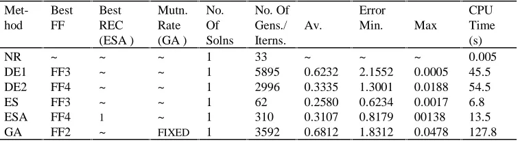
Table 5. Results For D Flip-Flop (C=D=R=S=1)

Met-hod

Best FF

Best REC (ESA )

Mutn. Rate (GA )

No. Of Solns

No. Of Gens./ Iterns.

Av.

Error

Min. Max

CPU Time (s)

NR ~ ~ ~ 1 33 ~ ~ ~ 0.005

DE1 FF3 ~ ~ 1 5895 0.6232 2.1552 0.0005 45.5

DE2 FF4 ~ ~ 1 2996 0.3335 1.3001 0.0188 54.5

ES FF3 ~ ~ 1 62 0.2580 0.6234 0.0017 6.8

ESA FF4 1 ~ 1 310 0.3107 0.8179 00138 13.5

The algorithms were tested using all the possible configurations. For example, ESA was tested using all the fitness functions and for each fitness function all the possible recombination operators were tried. Different parameter settings were also tried in an attempt to obtain optimum performance. The same approach to testing was applied to each algorithm, for each test circuit and where possible the most reliable configuration of input parameters of an algorithm was used to obtain a fair comparison. As a result, a large amount of test data was generated and could not practically be included in this paper. Hence, the tables contain the data for the best run of each algorithm on each circuit. Parameter settings have been omitted from the tables because they are generally those suggested in earlier sections but can vary slightly from problem to problem.

From the above tables we can see that NR is by far the quickest of all of the methods and in the majority of cases GA performs worst in terms of both speed and accuracy. GA was the most sensitive to parameter settings. The poor performance of GA is expected mainly because of the need for special representations of the solution vector components. The best choice of fitness function was FF4 or FF3. Even when FF1 or FF2 worked best, FF3 and FF4 were not far behind.

From these results, DE1 and DE2 give the best results in terms of the number of solutions found. Furthermore, DE1 and DE2 yield accurate results in the majority of cases, although the self-adaptive ES also has good accuracy. The CPU time for the algorithms can vary dramatically from circuit to circuit, sometimes as a result of small changes to input parameters. Hence, when using these methods one should weigh up whether speed is the most important point or whether getting multiple solutions is more important. Overall, DE (1 or 2) seems to be the best general evolutionary algorithm because they are very simple to implement, they are both compact code-wise and they also have the least memory overhead because of the small population size.

4.

C

The use of Evolutionary Computing algorithms for nonlinear operating point analysis of MOS circuits has been described. It has been demonstrated that EC and particularly Differential Evolution has some notable advantages over conventional NR. In principle, DE and the other EC algorithms are globally convergent, whereas NR is only locally convergent. It has been shown that DE can find multiple solutions in a single pass. It has also been seen that all of the EC techniques are sensitive, by varying degrees, to reproduction parameters, such as the mutation rate, population size, recombination strategies etc. The success of DE is partly due its self-adaptive nature and although DE uses mutation as a primary operator it also contains a recombination operator. Another excellent feature of the DE algorithms is that the population size is automatically scaled in proportion to the size of the given problem, which can help avoid over- and undersized populations. These features and the way they are implemented in DE have been the major contribution to DE’s good performance.

Evolutionary techniques are normally globally convergent but the quality of the solutions can vary. NR can diverge and is only locally convergent but the solutions are extremely accurate. It is reasonable to ask whether a hybrid method is possible so that we have the best of both worlds. Such a method has been proposed by Salomon [13] called

Evolutionary-Gradient-Search (EGS).

Future work will include devoting time to increasing the performance of the best algorithm, namely DE, in terms of convergence speed and accuracy. The next stage in development will require testing the DE algorithms on significantly larger circuits. This in turn will require a more sophisticated circuit simulator. The DE algorithm will, therefore, be integrated into such a simulator. This will be beneficial, firstly, because we will be able to build a much wider class of circuits and, secondly, we will see just how feasible EC is as a solution method for DC analysis of large circuits. The use of EC for other types of circuit simulation, such as Transient Analysis, will also need to be explored and can be included as part of the integration process into a SPICE-type simulator. Once this integration has been completed the main improvement to the EC method will be to reduce the CPU time, at present the EC algorithms are at best two orders of magnitude slower than NR.

R

[1] Ho, C.W., Zien, D.A., Ruehli, A.E. and Brennan, P.A., An Algorithm for DC Solutions in an Experimental General Purpose Interactive Circuit Design Program, IEEE Trans. on Circuits and Simulation, Vol. CAS-24, No. 8, August 1977.

[2] Broyden, C.G., A Class of Methods for Solving Nonlinear Simultaneous Equations, Math Comp., Vol. 19, 1965, pp 577-593.

[3] Najibi, T.N., Continuation Methods as applied to Circuit Simulation, IEEE Press Circuits and Devices Magazine, Vol. 5, No.5, 1989, pp 48-49.

[4] Trajkovic, L., Homotopy methods for computing dc-operating points in Encyclopedia of Electrical and Electronics Engineering, vol. 9, pp. 171-176, 1999, John Wiley & Sons. [5] Storn, R. and Price, K., Minimizing the Real Functions of the ICEC ’96 Contest by

Differential Evolution, Proceedings Int. Conf. On Evolutionary Computing, Nagoya. 1996

[6] Storn, R. and Price, K., Differential Evolution: A Simple and Efficient Adaptive Scheme for Global Optimization Over Continuous Spaces, Tech Report TR-95-012, ICSI, Berkeley, 1995 [7] Goldberg, D.E., Genetic Algorithms in Search, Optimization and Machine Learning, Addison

Wesley, 1989.

[8] Fogel, D.B., Evolutionary Computation: Towards a New Philosophy of Machine Intelligence, 2nd Ed., IEEE Press, NY, 2000.

[9] Fogel, L.J., Autonomous Automata, Industrial Research, Vol. 4, 1962, pp 14-19.

[10] Rechenberg, I., Cybernetic Solution Path of an Experimental Problem, Royal Aircraft Establishment, Library Translation No. 1122, August 1965.

[11] Bäck, T. and Schwefel, H.-P., An Overview of Evolutionary Algorithms for Parameter Optimization, Evolutionary Computation, Vol. 1:1, 1993, pp 1-23.

[12] Storn, R., On the Usage of Differential Evolution for Function Optimization, Technical Report, ICSI, Berkeley, 1996.