q2001 American Meteorological Society
Large-Scale Propagating Disturbances: Approximation by Vertical Normal Modes
PETER D. KILLWORTH ANDJEFFREY R. BLUNDELL Southampton Oceanography Centre, Southampton, United Kingdom
(Manuscript received 5 September 2000, in final form 29 January 2001) ABSTRACT
Propagating features and waves occur everywhere in the ocean. This paper derives a concise description of how such small-amplitude, large-scale oceanic internal disturbances propagate dynamically against a slowly varying background mean flow and stratification, computed using oceanic data. For a flat-bottomed ocean, assumed here, the linear internal modes, computed using the local stratification, form a useful basis for expanding the oceanic shear modes of propagation. Remarkably, the shear modal structure is largely independent of ori-entation of the flow. The resulting advective velocities, which are termed pseudovelocities, comprise background flow decomposed onto normal modes, and westward planetary wave propagation velocities. The diagonal entries of the matrix of pseudovelocities prove to be reasonably accurate descriptors of the speed and direction of propagation of the shear modes, which thus respond as if simply advected by this diagonal-entry velocity field. The complicated three-dimensional propagation problem has thus been systematically reduced to this simple rule.
The first shear mode is dominated by westward propagation, and possesses a midlatitude speed-up over the undisturbed linear first-mode planetary wave. The pseudovelocity for the second shear mode, in contrast, while still dominated by westward propagation at lower latitudes, shows a gyrelike structure at latitudes above 308. This resembles in both shape and direction the geostrophic baroclinic flow between about 500- and 1000-m depth, but are much slower than the flow at these depths. Features may thus be able to propagate some distance around a subtropical or subpolar gyre, but not, in general, at the speed of the circulation.
1. Introduction
Propagating features—of which waves are a subset— are ubiquitous in the ocean. They play an important climatic role, permitting information about changes in one region of the ocean to be transmitted to another. A variety of data sources now exists to demonstrate the existence of propagating features: historical hydro-graphic and XBT records, and remotely sensed sea sur-face temperature and sea sursur-face height. Hydrographic data, while inadequate for many purposes, have proven ideal for analysis of large-scale changes (White 1977 is an early example). They have been used in the North Atlantic to show interdecadal changes (Levitus 1989), and in the North Pacific (Jacobson and Spiesberger 1998) to show planetary waves. Deser et al. (1996) and Zhang and Levitus (1997) used EOF analyses on the new Levitus data to examine subsurface propagation in the North Pacific, seeing cold pulses moving downward from the surface (where they may well be initiated by atmospheric forcing) into the main thermocline, on in-terdecadal timescales. At depths of 250 m, the
move-Corresponding author address: Dr. Peter Killworth, Southampton
Oceanography Centre, Empress Dock, Southampton, SO14 3ZH, United Kingdom.
E-mail: [email protected]
ment appeared clockwise around the subtropical gyre plus a westward phase propagation, similar to sugges-tions of Latif and Barnett (1994).
in altimeter data. Chelton and Schlax (1996) produced the first global analysis and showed that the zonal speed was distinctly higher than that predicted by linear the-ory, though Kessler (1990) had found suggestions of this earlier in XBT data. [Zang and Wunsch (1999) have debated whether waves are in fact faster than linear theory.] However, planetary waves are not only visible in altimeter data. Cipollini et al. (1997) showed that in the Azores region they were clearly visible in infrared measurements of surface temperature, and Hill et al. (2000) have extended these observations to the global ocean. Cipollini et al. (2001) have made similar obser-vations with ocean color.
The Chelton and Schlax (1996) observations trig-gered much theoretical work. Killworth et al. (1997, henceforth KCdS) showed that the speed of the first baroclinic mode of propagation is mainly increased by the presence of (baroclinic) mean flow, through changes in the background potential vorticity, and gave the first proof of the noninteraction theorem; this was confirmed by Dewar (1998) and Liu (1999b). These latter papers, together with de Szoeke and Chelton (1999), gave ar-guments for why the increase in speed was found pre-dominantly in mid and high latitudes. Dewar and Morris (2000) have examined baroclinic wave propagation in an eddy-resolving flat-bottomed quasigeostrophic mod-el, finding modifications to wave speeds consistent with the above theories. Killworth and Blundell (1999) showed that the effects of basinscale topography on propagation were locally large, but globally small. The combination of the mean flow and topography has yet to be investigated.
Interest has moved recently toward higher modes, when they exist (e.g., Cipollini et al. 1997). Liu and Zhang (1999), using ray tracing in a 2.5-layer model of the North Pacific, showed that the first baroclinic plan-etary wave mode moved predominantly westward, but the second mode was advected by the mean flow. Ezer (1999) modeled decadal variability of the upper North Atlantic in the subtropics, finding cold temperature anomalies propagating eastward and downward, pos-sibly forced by the Gulf Stream.
We need to both understand the process by which features and waves propagate, and obtain good numer-ical predictions for that behavior. The situation for pas-sive tracers is simple: they are advected along mean streamlines. We therefore limit attention to dynamical features henceforth. These are not advected along mean streamlines under almost any circumstances, since if q is some conserved quantity [e.g., potential vorticity, as used by Zhang and Liu (1999), or potential temperature, etc.] with mean value q and perturbation q9, then q9 satisfies
q9 1t u9·=q 1u ·=q9 50 (1.1) so that anomalies are not simply advected byu (which would lie along q 5 const). Any description of the anomaly propagation must solve (some version of ) the
full three-dimensional problem. There are implicit dif-ferences in the roles of the horizontal and vertical in this problem, due to the existence of wave propagation dependant upon the mean vertical structure.
Understanding the behavior of (1.1) has not proven easy. It is fully three-dimensional, so that use of a sim-plified numerical model (e.g., frictional planetary geo-strophy, which can handle both mean flow and topog-raphy) or a full general circulation model, while sim-ulating propagation of disturbances, does not yield easy
insight into the dynamics of the disturbances. Such
in-sight involves some simplification, particularly of the vertical aspect of the problem, without losing accuracy [though rays can be traced three-dimensionally, e.g., Yang (2000)]. The quasigeostrophic approximation re-quires a spatially uniform stratification, which is not useful if our aim, as here, is to describe propagation on basin scales. Simplifications such as 1.5- and 2-layer models give understanding but will not be reliable for calculations in the real ocean. Indeed, Flierl (1978) ar-gues cogently that layered models need calibration be-fore they yield useful results, and recommends the use of modal decomposition instead. This approach—but using vertical normal modes appropriate to the local stratification, and that vary slowly in the horizontal— will be employed here. The concept is basically WKBJ: the background circulation and stratification vary on the basin scale, while the (geostrophic) waves vary on scales much shorter than the background. The sole dis-advantage of casting onto vertical normal modes is that the correct bottom boundary condition for varying to-pography cannot be handled with any accuracy using normal modes. In this paper we therefore use the flat-bottom boundary condition [cf. Killworth and Blundell (1999) for a proper treatment in the absence of mean flow].
pseudoveloc-ity remains stubbornly westward in all locations, but at latitudes above 308, the second shear mode propagates in directions resembling, but not identical to, the mid-depth (500–1000 m) baroclinic background flow, and at somewhat slower rates.
2. Normal-mode decomposition
The equations of motion are now cast onto a single variable M, using Welander’s (1959) notation. This uses the planetary geostrophic approximation, which permits variation of background stratification (unlike the qua-sigeostrophic approximation), though only for geo-strophic flow. For simplicity only, the analysis is pre-sented on a Cartesian plane. All data analysis and com-putations in this paper are, however, performed using full spherical geometry. In terms of M, we have
M
p gr zy
Mz5 ; Mzz5 2 ; u5 2 ;
r0 r0 f
Mzx b
y 5 ; w5 2M ,x
f f
where the symbols have their usual meaning, andb 5
fyis not necessarily constant. When substituted into the
conservation of density (rt1 u ·=r 50) we obtain
M Mzy zzx M Mzx zzy b
Mzzt2 1 1 2M Mx zzz5 0. (2.1)
f f f
As explained earlier, we can assume M (2H )50, which is the flat-bottom boundary condition corresponding to zero vertical velocity. (Recall that varying bottom depth cannot be attacked easily with normal modes.) We now pose a small perturbation M9to the mean flowM. The latter is assumed a function of all three spatial coordi-nates; Pedlosky (1987) discusses the effects this may have on the small perturbations from the aspect of the instability problem. In what follows, bothM and M9are assumed to vanish at the surface z50. The former will not be true in general, but the additional barotropic com-ponent can be added in later, as will be shown. The vanishing of M9at the surface corresponds to unforced propagation or free waves. The linearized system be-comes
1 1
M9 2zzt (M Mzy 9 1zzx M9zyM )zzx 1 (M Mzx zzy9 1Mzx9M )zzy
f f
b
1 2(M Mx zzz9 1M9xM )zzz 5 0.
f (2.2)
We now make the fundamental approximation for this paper, standard for the WKBJ theory to be used later, that
Lpert
Lbasink Lpertka; or 5 « K1, (2.3)
Lbasin
where Lpert, Lbasinare length scales for the perturbation
and the mean flow, respectively, and a is the deformation radius. All aspects of the mean flow (including the strat-ification) vary with length Lbasin. The perturbation scale
Lpert is, however, not small enough for the assumption
of geostrophy to fail, by the second half of (2.3). The approximation (2.3) permits rather more progress than is usual within WKBJ theory. In practice—as with al-most any scale separation theory—there are areas in the World Ocean in which the background flow changes sufficiently rapidly to invalidate (2.3), more usually in the north–south direction. However, experience with WKBJ theory suggests that such theory continues to give useful results even when (2.3) is not well satisfied. In the wave propagation cases considered here, the de-pendence of east–west phase speeds on latitude means that short north–south scales develop in the solution, helping to mitigate the more rapid north–south variation of the mean flow.
In (2.2), then, the first term in the last parentheses is formally smaller than the second by an amount O(«). Henceforth, this term is omitted; its inclusion makes negligible changes to the results.1Another, more useful,
way to write (2.2) is
2
bN
M9 1zzt u ·H =M9 2zz uHz·=M9 1z 2 M9 5x 0, (2.4)
f
where the suffix H denotes the horizontal component, and we have written Mzzz 5 N2(x, y, z). Due to
geo-strophy, (2.4) is equivalent to the long-wave assump-tion.
We now seek to simplify the fully stratified problem above. This is frequently done using a layered decom-position. However, Flierl (1978) pointed out that casting onto normal modes gave a considerably more accurate representation of dynamics, at least in the quasigeo-strophic regime he considered. Accordingly, we cast (2.4) onto the normal modes for a background density stratification given by a buoyancy frequency N2(x, y,
z). The normal modes are
2
N
hˆj(x, y, z): hˆjzz1 2hˆj5 0; hˆ 5 0,
Cj
z5 0, 2H(x, y).
(2.5) Here Cjis the internal wave speed of the jth eigenmode.
The equivalent basis function for horizontal velocity is
uˆi(x, y, z)5hˆiz. The hˆ, uˆ are normalized at all points by
0 0
2 2
N hˆ hˆ dz5HCd; uˆ uˆ dz5Hd (2.6)
E
i j i ijE
i j ij2H 2H
so that hˆhas units of length and uˆ is dimensionless. The
1The neglected term is in fact much smaller than the simple scaling
sign convention is such that all the uˆ are positive at the surface. Progress will be possible because the hˆ, uˆ vary
only slowly across the basin with scale Lbasin, while the
perturbation fields vary on the more rapid scale Lpert.
We expand the background (now only horizontal) mean velocity in the uˆ and the M9in the hˆ:
`
uH 5
O
u (x, y)uˆ (x, y, z);k k k51`
M9 5
O
M9k(x, y, t)hˆk(x, y, z) (2.7)k51
(recall that we can add in the mean barotropic com-ponent later, so the first sum starts from 1).
The mean quantities can easily be calculated from data. AssuminguHis known from density data and the
use of the thermal wind relationship, the orthogonality condition implies
0
1
uk5
E
u uˆ dz.H k (2.8)H 2H
We now note that all horizontal and time derivatives in (2.4) act on the perturbation quantity M9. From the sec-ond part of (2.7), we have, for example,
`
M9 5x
O
{Mkx9hˆk1 M9khˆkx}.k51
In this sum, the first terms involve derivatives on the rapid (Lpert) scale, while the second involve derivatives
on the slower (Lbasin) scale. Accordingly, the derivatives
of M9dominate over those involving horizontal
deriv-atives of the basis functions hˆ, so that the latter may be
neglected. In other words, casting onto local modes and neglecting their slow lateral variation is legitimate with-in the scale assumption (2.3).
Substituting (2.7) into (2.4) gives, neglecting terms as just demonstrated,
2 2 2
N N N
2
O
M9jt 2hˆj1OO
5
2u hiˆizMjx9 2hˆj2yihˆizM9jy 2hˆj6
C C C
j j i j j j
2 2
N N
1
O O
5
uj 2hˆjM9ixhˆiz1 yj 2hˆjM9iyhˆiz6
C C
i j j j
b 2
1 2
O
M9jxhˆjN 5 0,f j
(2.9) where (2.5) has been used for second derivatives of hˆ.
Multiplying by hˆk and integrating top to bottom, we
obtain, using orthogonality and multiplying by21/H,
aijk
M9 1kt
O O
2{u Mi jx9 1yiMjy9 2u Mj 9 2ix yjM9iy}C
i j j
b 2
2 2C Mk 9 5kx 0.
f (2.10)
Here the triple interaction coefficient
0
1 2
a 5ijk
E
N hˆizhˆjhˆk dz (2.11)H 2H
is a dimensional equivalent to that defined in KCdS. Note thatais symmetric in its last two suffixes. Flierl (1978) used similar coefficients in the quasigeostrophic regime.
The last term in (2.10) is simply westward advection of mode k by the kth internal planetary wave speed / f2. The remainder of the equation can be further 2
bCk
simplified by defining the dimensionless interaction co-efficient
ajki akji
g 5ijk 2 2 2, (2.12)
Ck Cj
which is antisymmetric in its last two suffixes. Then we write the sum
eff
ukn 5
O
umgkmn (2.13)m
and substitute into (2.10), obtaining
b
eff eff 2
M9 1kt
O
{u Mkn 9 1nx yknM9ny}2 2C Mk 9 5kx 0. (2.14)f
n
By defining
b
net eff 2 net eff
ukn 5 ukn 2 2Ckdkn; y 5 ykn kn (2.15)
f
(2.14) becomes
net net
M9 1kt
O
{u Mkn 9 1nx yknMny9} 5 0, (2.16)n
which is a coupled set of advective equations for the componentsM9k.
Thus, the vector of modal contributions M9k is ad-vected by a set of pseudovelocities, obeying the simple (horizontal) advection rule
net
Mt1 U ·=M 5 0, (2.17) where M is the column vectorM9k and
net net net
U 5 [u ,kn ykn]. (2.18) It is of interest to examine a single mode, R, say. From (2.16),M9Ris advected by all internal modes. In partic-ular it is self-advected throughueff. From (2.13), this is
RR
SiuigRiR. The antisymmetry in the last two components
ofgshows that the only background velocity mode that does not contribute to this sum is the Rth mode itself. This is another demonstration of the non-self-interaction theorem for geostrophic normal modes, first shown for continuous stratification by KCdS; see also Liu (1999b) for a discussion in the finite layered system.
Addition of the background barotropic mode, if re-quired, is now straightforward. Since it has no density signature, it merely adds an extra term uBdkn to the
term, where uB is the depth-independent velocity,
eff ukn
FIG. 1. The zonal average of the vertical maximum of | u | and |y| as functions of longitude. At all locations the maximum of | u | is much larger than that for |y| . Values within 58of the equator are not shown.
The sums above are formally infinite. In practice, there will be truncation. This can happen in two inde-pendent ways. First, the number of modes K included in the sum (2.13) to obtain ueffis chosen. Second, the
number of terms in the sum (2.17) for the evolution equation, L, say, can be chosen such that L # K; for
example, one could imagine computingueffusing many
11
modes but only retaining that single term in (2.17) as an approximant.
3. Computation of the pseudovelocities
The pseudovelocities unet, ueff were computed from
kn kn
annual-mean temperature–salinity data for the World Ocean (Levitus and Boyer 1994; Levitus et al. 1994) on a 18horizontal grid. These were analyzed to produce local values of N2, u
z, and yzas functions of depth at
the standard depths. The baroclinic u and y are then obtained by integration plus the requirement of no net vertically integrated horizontal flow. The precise loca-tion of the ocean floor was taken from an averaging of the 5-minute gridded Earth topography data set, ETO-PO5 (National Geophysical Data Center 1988), onto the same grid.
The no-mean-flow eigenproblems are solved as ma-trix eigenvalue problems, ordered by westward phase speed. In most cases, at least the first four eigenvalues and vectors are retained in what follows.
a. The background velocity modal loadings ui
These computations, en route, demonstrated a fact that to our knowledge has not been noted previously. At each horizontal location, the minimum and maximum of u and y were computed within the fluid column. Because the flow is defined to be baroclinic, the
mini-mum (maximini-mum) is negative (positive). For each flow direction, the minimum and maximum were combined to give the maximum modulus of the flow in that di-rection. The average of these moduli around a latitude band is plotted in Fig. 1. Throughout the paper, we concentrate on the latitude range 6508, since turning latitudes for planetary waves of annual frequency are of this order. The zonally averaged speeds are a rea-sonable proxy for the full fields over most of the deep ocean.
The north–south flow is seen to be much weaker than the east–west flow on average at all latitudes. It is also smaller in 89% of the 18 3 18 ocean squares between
65 and6508, and indeed the maximum modulus north– south flow is less than half the east–west equivalent in two-thirds of these squares. (The north–south flow is larger within a few degrees of eastern and western boundaries in most oceans, and in a few isolated mid-latitude locations in the North Atlantic and Southern Oceans. This ignores the main western boundary cur-rents, since these are sited over shelf-slope regions. We have excluded such regions, using a cutoff depth of 1000 m, from this essentially deep ocean theory because the assumptions underlying a modal treatment become in-appropriate.)
The reason for mainly weaker north–south flows is the relative width of most ocean basins compared with the north–south distance over which surface density changes owing to atmospheric forcing. The atmosphere itself is, of course, an example in which neglect of x variation can be a reasonable approximation. While this cannot be exactly true in the ocean, theories have been worked out for zonally invariant basins (e.g., Welander and Liu 1976).
Ifyis in some sense ‘‘small’’ over most of the ocean compared with u, then the majority of advective-influ-enced flows will tend to be oriented east–west, so that propagation of disturbances around a gyre is made more difficult. However, though y is mainly small, the ex-tended width of typical midlatitude basins means that even a small north–south velocity can be associated with significant latitudinal migrations under suitable circum-stances.
The relative smallness of y is also indicated in Fig. 2, which shows the longitudinal average of the modal decomposition of the background u andyfields for the first four modes. The values are clearly dominated by
u1 (recall that this does not yet include the planetary
wave b term), with values of order 1 cm s21 in most
regions, becoming largest in the Antarctic Circumpolar Current and near the equator. The values of u2 and u3
are much smaller than u1; recall that KCdS showed that
it was the second internal background east–west mode—
u2 in this notation—that was responsible for much of
FIG. 2. The zonal average of modal coefficients (a) u1,y1, u2,y2
and (b) u3,y3, u4,y4as functions of latitude. Values within 58of the
equator are not shown.
TABLE1. Values of Unet(cm s21) at 35.58N, 150.58E (North Pacific).
The bold items are values that should be theoretically small in most places. For shear mode 1, the east–west phase speed computed from the vertically stratified problem is23.7 cm s21, and that from the 4 34 matrix (computed with K54) given is also23.7 cm s21. The
eigenvalue from the 232 submatrix is23.3 cm s21. The mode 1
and 2 loadings for the eigenvector are 0.99 and 0.13, respectively. For shear mode 2, the stratified phase speed is21.3 cm s21, and that
from the 434 matrix is20.8 cm s21. The eigenvalue from the 2 32 submatrix is20.6 cm s21. The mode 1 and 2 loadings for the
eigenvector are 0.82 and 0.56, respectively.
u : i/jnet
ij 1 2 3 4
1 2 3 4
25.2
21.2
20.8
20.3
7.2 1.3
0.8
20.1
6.1 5.8 3.0
1.8
1.2 3.3 5.7 4.2
ynet: i/j
ij 1 2 3 4
1 2 3 4
20.2
20.0
20.0
20.0
20.6
20.3
20.1 0.0
20.1
20.5
20.3
20.1
20.2 0.1
20.4
20.4
is positive; it will turn out that this is in competition with the westward propagation of mode 2, permitting a second mode to move more freely north–south.
The coefficientsy1,y2take the signs given from east–
west thermal wind applied to warm poleward western boundary currents and colder equatorward interior flow. The higher modes are uniformly small, so that the trun-cation of the total number of modes computed (K in the above notation) can be at a small value—we shall typ-ically use 2—without loss of accuracy. Put another way, the values ofunet,ynetare mainly independent of K,
pro-kn kn
viding K $ 2.
b. The values of the pseudovelocitiesunet
kn
We turn now to consideration of the pseudovelocities themselves. From (2.13), these are sums of the ui,
weighted by the g coefficients. These latter are
com-puted in situ from the vertical structure, but in fact do not differ strongly from place to place. If an approximate WKBJ form is used for the vertical normal modes (cf. KCdS, p. 1963, for the first mode; the others are similar) then it is straightforward to show that (i) gabc is only
sizeable if in some order a 5 b1 c, and (ii)gabc
de-creases as min (a, b, c) inde-creases. Point (i) is because the stretched sinusoidal nature of the eigenvectors means that the triple integrals to obtainaijk, and hence
gijk, have reasonable nonzero values only when sums
and differences of sinusoids interact. Point (ii) is be-cause the increasingly oscillatory nature in the vertical as the mode number increases means that the integrals naturally decrease. These remarks hold reasonably well for low orders.
Combining this information with the previous find-ings that high modal loadfind-ings uiare small puts strong
restrictions on the coefficientsunet. The diagonal east–
kn
west terms will be large due to thebterm, though this decreases rapidly with mode number. In particular, the first column below the diagonal will generally be small, since ueffk1 is Sm umgkm1. The m 5 1 term in this sum
vanishes since gk11 is zero. The remaining terms only
involve um, m . 1 and so are smaller in magnitude.
The second column above the diagonal (ueff) can be a
12
reasonable size since it involvesg112u1. The remainder
of the second column, below its diagonal, is mainly small for similar reasons, save forueff, which involves
32
g312u1, neither term of which is necessarily small.
Similar arguments extend to higher rows and col-umns: values above the diagonal can have reasonable sizes, while those below tend to be small. Two typical instances are shown in Tables 1 and 2, which show the 434unetcoefficients (i.e., including the planetary wave
kn
TABLE2. Values of Unet(cm s21) at 40.58N, 35.58W (North Atlantic).
For shear mode 1, the east–west phase speed computed from the vertically stratified problem is21.2 cm s21, and that from the 43
4 matrix (computed with K54) given is21.1 cm s21. The eigenvalue
from the 232 submatrix is20.9 cm s21. The mode 1 and 2 loadings
for the eigenvector are 0.98 and 0.20, respectively. There is no real stratified phase speed for shear mode 2. That from the 434 matrix is20.8 cm s21. The eigenvalue from the 232 submatrix is10.3
cm s21. The mode 1 and 2 loadings for the eigenvector are 0.93 and
0.37, respectively.
u : i/jnet
ij 1 2 3 4
1 2 3 4 21.7 20.4 20.3 20.1 2.2 20.0 0.4 20.1 2.1 1.7 1.0 0.6 0.2 0.4 1.9 1.3
ynet: i/j
ij 1 2 3 4
1 2 3 4 20.1 0.1 0.1 0.1 20.4 20.0 20.1 0.0 20.1 20.4 20.3 20.1 20.2 0.1 20.4 20.3
North Atlantic. The sizes are in good agreement with the arguments presented here.
In the particular case of a 23 2 truncation, ueff
be-kn
comes simply
2g112u2 g112u1
,
[
2g212u2 g212u1]
where theg coefficients shown are both positive. Over latitudes between65 and6508, on averageg11252.54,
andg21250.83. Note that the term is proportional eff
u22
to u1. This is positive at mid- and high latitudes, as
noted previously. As the size of the planetary wave correction decreases with distance poleward, at some latitude it may be possible forueffto become positive;
22
that is, the background flow may be sufficient to alter the propagation velocity for the second mode from west-ward, its natural direction, to eastward.
These predictions are confirmed by Fig. 3, which shows longitudinal averages of the (vector) 232 com-ponents of the Unet matrix.2 [There is no ideal way to
show these data due to the large variation in size. An alternative (Fig. 4) shows longitudinally averaged
mod-uli of the (vector) 232 components of the Unetmatrix.
Moduli are used since the strong planetary wave com-ponent makes the diagonal u terms dominant save at high latitudes; the strong value ofunetnear the equator
11
requires a logarithmic scale to show detail at higher latitudes.] Either presentation shows again that the above-diagonal terms are not negligible, while the be-low-diagonal—here only the (2,1) term—tends to be small. As in the modal casting of the background ve-locities, u dominatesyalmost everywhere. As predicted, poleward of about 358, ueff is positive (though only a
22
few millimeters per second in the Northern Hemi-sphere), raising the possibility that anomalies may be able to propagate with an eastward, rather than west-ward, component.
4. Shear modes
The behavior of the advective modal system (2.17), or of the original continuously stratified problem (2.2), is generally complicated. For the moment, we write Mi
as a horizontal Fourier decomposition with wavenumber
k 5 (k, l ) and frequencyv:
i(kx1ly2vt)
Mi5
EE
a (k, l)ei dk dl. (4.1)If the velocity field were horizontally uniform, or if using a WKBJ formulation, assuming as before that the background fields vary on the length scale LbasinkLpert,
then each Fourier mode would satisfy an eigenvalue relationship
2These terms were computed using a four-mode expansion, but
almost identical answers occur with two, three, or more than four modes included.
net
(k · U )M5 vM, (4.2)
where M represents the vectorM9i.Modes that satisfy (4.2) we term ‘‘shear modes,’’ oriented along (k, l ), using Killworth and Anderson’s (1977) terminology. They are the natural vertical structures (or, here, modal structures) that can propagate locally. Equation (4.2) is an implicit dispersion relation for the waves. To be solved, the number of modes would be truncated. If the decomposition (2.16) is truncated at L modes (with L # K ), the eigenvalue relation becomes the matrix
re-lation
L
net net
(ku 1ly )M9 5vM9, i51, 2, · · · , L. (4.3)
O
ij ij j i j51Since the matrix operator in (4.3) is not symmetric, the shear modes are not orthogonal. In the continuously stratified problem, we set M9 5F(x, y, z) expi(kx1ly 2 vt), where F is a slowly varying function of the
horizontal, and obtain
2
bN
(ku1ly 2 v)Fzz2(kuz1lyz)Fz1 2 kF50 (4.4)
f
together with boundary conditions
F(0)5 F(2H)5 0 (4.5)
since we restrict attention to a flat bottom. The system [(4.4), (4.5)] is not self-adjoint, though progress can be made, as will be shown elsewhere. The solutions of KCdS are the first shear mode for the continuous prob-lem, oriented east–west.
Both systems can yield real or complex eigenvalues, the latter corresponding to long-wave instability (cf. KCdS; Liu 1999a for discussions). Over the World Ocean between 6(5–50)8, a negligible 0.08% of 18 squares possess no real shear mode solutions to the 4
FIG. 3. Zonal averages of pseudovelocitiesunet,ynetfor (a) k, n5
kn kn
1,1; 1,2 and (b) k, n52,1; 2,2. Values within 108of the equator or above 0.20 m s21in magnitude are not shown.
FIG. 4. The zonal average of |unet| , |ynet| for (a) k, n51,1; 1,2
kn kn
and (b) k, n52,1; 2,2. A logarithmic scale is used so as to show high-latitude detail that would otherwise be swamped by near-equa-torial values. Values within 58of the equator are not shown.
shear mode solutions (the remainder of the squares, 73%, having the full four real solutions). (The 3 3 3 solutions yield similar figures, e.g., 82% squares with all three real solutions. The 5 3 5 solutions are again similar, though now 99% of the solutions have at least three real shear modes, so that some details of the reality of the solutions depend on the truncation used.) Al-though around 28% of 18squares possess some complex solutions, with L $ 4 there remain at least two real solutions (corresponding to the gravest shear modes) in these locations. So at least the first two shear modes can propagate throughout the ocean, but higher shear modes will move into regions where there potentially is growth or decay at small wavenumbers. Such areas are not eas-ily treated with WKBJ analysis, since there will typi-cally be caustics surrounding the areas of complex so-lutions, and linkage techniques must be employed to cross the real–complex boundary.
The small number of complex modes does, however, remain interesting. A referee raised the question of whether the number might be underestimated because of a singular limit, due to the order in which the limits are taken in the usual baroclinic instability problem (the background relative vorticity is neglected, and the per-turbation wavenumber is set to zero for the geostrophic problem). While we have not investigated this fully, we do not believe that any singular limit can occur. First, the limit that neglects background relative vorticity can occur independently of the perturbation length scale be-ing large compared with a (in our case, this neglect is doubly justified because the background flow varies on the basin scale only, so that the relative vorticity, of order U/L2 , is negligible compared with b, which is
basin
retained). Second, Fu and Chelton (2001) have com-puted the non-long-wave solutions for a background east–west flow and found that the problem is fully con-tinuous in the geostrophic limit.
FIG. 5. The variation of modal amplitudes present in the first four shear modes at 35.58N, 150.58E, as the orientation of the wavenumber is altered. The values were computed at multiples of 28; between 808and 1008at least one shear mode is not present, and so none are shown.
shear modes in the 434 matrix case are mainly located at high latitude (specifically in the Antarctic Circum-polar Current) and with occasional latitudinal bands (e.g., around 208N in the Pacific). In the 5 3 5 case, the areas of two unstable shear modes are similar; how-ever, the third shear mode is now stable there. We shall concentrate almost exclusively on the first two shear modes henceforth, so that complex solutions are not an issue.
The continuous problem [(4.4), (4.5)] in general has a finite number of solutions, the number decreasing as the magnitude of the mean flow increases. The decom-position approach, however, always possesses L solu-tions. This is a familiar problem. For example, if one poses the one-dimensional continuous Eady problem, which has two solutions, either as a finite-difference
problem with K points or by casting it onto K internal modes, then K apparent solutions will be found, all but two of which are numerical in nature.3Thus, we expect
that not all the modal behavior—or by analogy, the be-havior of an K-layered system—will be a good approx-imation to the behavior of the original stratified system. Appendix A gives a specific, though not realistic, ex-ample (when the east–west wavenumber k50) in which the modal decomposition gives incorrect solutions.
At any event, the propagation of a large feature in-volves more complexity than the simple (4.3). This ei-genvalue relation clearly depends on the orientation of
3The continuous Eady problem has delta-function solutions,
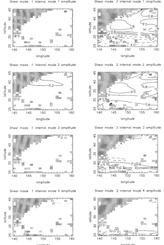
FIG. 6. The modal amplitudes of the first two shear modes in the Northwest Pacific, with east– west orientation, as determined from a four-mode decomposition. The contour interval is 0.2; negative contours dashed, zero contour dotted. Gray areas denote land (in the northwest corner) or regions where a real (stable) shear mode cannot be found.
the wave vector. It does not depend, other than a simple rescaling ofv, on its magnitude, due to the original
long-wave assumption, a feature shared by the continuous problem. Even if the entirety of a feature were describable by a single vertical structure, this structure would not necessarily be the eigenstructure for all wavenumber
[image:10.612.133.471.75.580.2]ori-entations and so would tend to spread as it propagated. Thus, whether a feature can maintain its shape depends on how sensitive the eigenvector solutions to (4.3) are to orientation of the wavenumber vector.
[image:10.612.318.463.88.190.2]FIG. 7. Comparisons of east–west oriented phase speeds (m s21) of shear mode 1 between the full continuous
local vertical calculation, the shear mode based on decompositions using two internal modes (that with three or more is indistinguishable), and the simple identification ofunetwith shear mode 1. The scatterplots are
11
over all (global) points with real solutions in the latitude range6(58–508). (a) The full calculation against the shear mode. (b) The full calculation againstunet. (c) Replots of (b), limiting attention to smaller phase
11
velocities by restricting the latitude range to6(308–508).
solutions to (4.3)] depends on the orientation of the wavevector at one location; the figure is typical of most midlatitude locations. Solutions are presented in terms of an eigenspeed v/ | k | , where k 5 | k | (cosf, sinf), rather than the less easily interpreted frequencyv. We
solve (4.3) using four modes as f varies between 08 and 1808(beyond 1808the sign of the problem is merely changed). The shear modes are ordered on the eigen-speed from the most negative, so that shear mode 1 at orientation 08 would be the fastest westward-propagat-ing mode as discussed for the continuous problem by KCdS.
The results show that the loadings of individual modes are remarkably invariant to orientation in this long-wave limit, other than occasional mode switches (e.g., the shear mode 2 and 3 exchange at around 408 orientation in the example). Shear mode 1 is dominated almost exclusively by internal mode 1 at all orientations, showing that the approximation used by KCdS (p. 1962) of replacing the shear mode by the internal mode was valid. Internal mode 1 is still mainly dominant in the second and third shear modes, although internal mode
2 becomes of similar importance. All four internal modes used have similar loadings in shear mode 4.
Near 908orientation, the number of modes decreases rapidly, and so values are not shown between 808and 1008orientation.
Appendix B gives approximate arguments based on the smallness of y compared with u that indicate that this invariance to orientation should be expected for both pseudovector and continuous representations.
The second factor that might act to prevent coherent propagation is if the shear mode changed its shape rap-idly in the horizontal. (Within a WKBJ framework this cannot happen: the shape is part of the slowly varying structure. However, a large feature, to be recognizable as such from data, needs to be horizontally coherent across Lpert.) Figure 6 examines how the internal mode
changes in shear mode 2 (and higher shear modes, not shown), but north of about 328there is little change in modal loadings, even in these shear modes. Thus, at such latitudes it is reasonable to expect that, to a good degree of approximation, a single shear mode can be coherent over the scale of a feature and can propagate following the solution of (4.3) while slowly changing its vertical shape in a WKBJ-like fashion.
5. Strongly truncated representations
Starting with the continuous system (2.2), the prob-lem has reduced successively to an infinite or finite ma-trix advection system for a collection of modes, and
then to an eigenvalue problem for propagation at a spe-cific angle. At all times through this procedure numer-ical solutions could be sought, and will be shown in a companion paper. In terms of understanding the prop-agation of baroclinic features, however, even the eigen-value problem is not of itself enlightening. We therefore seek further simplifications, by truncating the matrix system heavily.
Such truncations give worthwhile results because of the arguments in section 3. There it was argued that diagonal terms in Unet—and hence in k · Unet—are large,
and above-diagonal terms may be large, but below-di-agonal terms are mainly small. The solution to the ma-trix eigenvalue relation (4.3) for some reasonably large number of modes is thus
net net net net net net
)ku11 1ly 2 v11 ku12 1 ly12 ku13 1 ly13 · · ·)
)
kunet1 lynet kunet1 ly 2 vnet kunet1 lynet · · ·)
21 21 22 22 23 23
) net net net net net net )5 0, (5.1)
ku31 1 ly31 ku32 1 ly32 ku33 1 ly 2 v33 · · ·
)
)
) • • • • • • • • • · · ·)
where boldface indicates values which tend to be small. This determinant can be expanded approximately down the first column as
net net
(ku11 1 ly 2 v11 )
net net net net
)ku22 1 ly 2 v22 ku23 1ly23 · · ·)
) )
net net net net
) )
3 ) ku32 1 ly32 ku33 1 ly 2 v33 · · ·)
) • • • • • • · · ·)
1 (small)5 0. (5.2)
Continuing to expand, we have approximately
net net net net
(ku11 1 ly 2 v11 )(ku22 1 ly 2 v22 )
net net
3 (ku33 1 ly 2 v33 ) · · · 5 0. (5.3) This gives approximate solutions
net net
v 5i kuii 1lyii , i5 1, 2, 3, · · · , (5.4) which is simple horizontal advection by the ith diagonal entry of Unet. (This would not be expected to hold for
all shear modes, since complex solutions would enter at some stage.)
a. The first shear mode
Equation (5.4) predicts that the gravest shear mode is approximately advected by (unet,ynet). This is
consis-11 11
tent with the findings of KCdS, [their Eq. (22)], who showed to a good approximation (for east–west prop-agation, but now seen to be more general) that there was an effective Doppler shift from the resting planetary wave speed by an amount proportional to the second background mode, precisely equivalent toueff.
11
The eigenvector corresponding to this can be evalu-ated approximately. Since modal loadings fall off rap-idly after mode 2, we here consider only the first two modes. We use the shorthand
net net
rij5 kuij 1 lyij
and note that r21can be considered small compared with
the other entries by the previous arguments. The solution of | r2vI | 50 is then approximately (5.4), but show-ing the small corrections:
r r12 21 r r12 21
v 51 r11 1 ; v 52 r222 .
r112 r22 r112 r22
The first eigenvector is then to the same degree of ap-proximation,
1
M15 r ,
21
[
r 2r]
11 22
and this, given the smallness of r21, is approximately
the vector (1, 0)Tand so is dominated by the first internal
mode. The entries in Tables 1 and 2 for east–west ori-entation give some detail. The continuously stratified first shear mode velocity in Table 1 is 23.7 cm s21,
which is also the eigenvalue from the 4 3 4 matrix shown; that for the 2 3 2 submatrix is 23.3 cm s21,
which is very similar. However, at this location the is less accurate, at25.2 cm s21. (As we shall see, net
u11
approxi-FIG. 8. As Fig. 7, but for phase speeds of the first shear mode oriented at 458to the eastward direction, and using the identification ofunetcos451ynetsin45 with shear mode 1.
11 11
mate approach of KCdS. The Table 2 results have sim-ilar properties, even to the overestimation of the shear mode speed by unet. This mode is similar to the graver
11
mode in two-layer models such as Liu’s (1999b) ‘‘non-Doppler-shift’’ mode, and has connections with char-acteristic velocities in such models (e.g., Luyten and Stommel 1986).
These examples notwithstanding, on a global basis is a superior estimate of the phase speed than the
net u11
matrix eigenvalue solution, for reasons that are unclear. Figure 7 shows scatterplots comparing (between lati-tudes 58–508from the equator) the exact continuous first shear mode phase speed with either (Fig. 7a) the 2 3 2 eigenvalue phase speed (that using more modes is indistinguishable) or (Fig. 7b) unet. Because the high
11
speeds near the equator are included, all correlations are near unity. Figure 7c, restricted to the latitude range
6(308–508), shows that at low speeds the correlations are less good: between continuous and shear mode the correlation is 0.5, and between continuous andunetit is
11
0.9. It should be noted that u11tends to overestimate the
phase speed. (KCdS show a similar result for model data.)
Figure 8 shows a similar diagram for propagation at 458 in the eastward direction. The phase velocities are now much reduced (as they are in classical planetary wave theory, so that the phases move east–west at sim-ilar speeds to before). The scatter at low speeds shown by the shear mode phase speed remains, with many eastward speeds not found in the full calculation. The superiority ofunetcos451ynetsin 45 to the shear mode
11 11
is similar to the case of eastward orientation, with a similar degree of overestimation.
b. The second shear mode
From (5.4), an approximation for the second shear mode phase speed would be (unet,ynet), again acting as
22 22
an effective Doppler shift to the undisturbed phase speed. The eigenvector would then take the approximate form
2r12
M25
1
2
r112 r22
[image:13.612.141.476.339.684.2]FIG. 9. As Fig. 7, but for the second shear mode, and using the identification ofunetwith shear
22
mode 2.
This is confirmed by the entries in Tables 1 and 2: the second shear mode does not take the form of the second internal mode, but possesses large loadings from the first internal mode. The mode 1 loading means that it may be possible for shear-mode-1-like behavior to ‘‘leak’’ faster disturbances westward from a slightly un-balanced second shear mode.
Tables 1 and 2 also indicate that the above approxi-mation is less good than for the first shear mode (indeed, no continuously stratified shear mode was located at the location in Table 2). Figure 9 confirms this. There is somewhat more scatter between the 2 3 2 eigenvalue and the full continuous problem than for the first shear mode. Over the full latitude range,unetserves as a valid
22
estimate. At low speeds (Fig. 9c) over substantial areas of the ocean a positive velocity is predicted, although most points are well correlated with the continuous so-lution. This mode identifies roughly with Liu’s (1999a,b) ‘‘advective,’’ or ‘‘A,’’ mode.
6. Propagation behavior
The previous section has shown that the diagonal pseudovelocities give reasonable, but not perfect, esti-mates of the propagation speed for a shear mode, for wavenumbers oriented in any direction save near 908(a rare occurrence in practice). Unfortunately, since most
propagation seems to occur at latitudes above 308, it is the slower speeds estimated by the pseudovelocities that contain more scatter, since the domination of the plan-etary wave speed over the background velocities be-comes less at higher latitudes. Appendix B gives ar-guments for why the shear mode propagation should resemble that of a single velocity vector, based on the smallness of ycompared with u in most of the ocean.
Figures 10 and 11 show the speeds and directions of propagation of the first two modes for the North Atlantic and North Pacific, respectively. The fields have been interpolated using the methods and software of Fieguth et al. (1998). Because the amplitude of the velocities differs strongly between high and low latitudes, it is hard to show detail at higher latitude. To aid this, ve-locities are not shown south of 158N, and the square root of the velocity (correctly oriented, taking cosine shrinkage of longitude and diagram aspect ratio into account) is shown rather than the velocity itself.
FIG. 10. Diagonal entries of the pseudovelocity matrix (i.e., estimates of the speed and direction in which free shear modes propagate) for the North Atlantic. The pseudovelocities have been interpolated using the Fieguth et al. (1998) software. Although computed on a 18grid, velocities are only shown every 28for clarity. Velocities are not shown south of 158N, and the square root of the velocity amplitude is shown, so that detail is visible in the small velocities at higher latitudes. The orientation takes the diagram aspect ratio and longitudinal convergence at higher latitudes into account. (a) The first shear mode pseudovelocities (unet). (b) The second shear mode pseudovelocities (unet).
11 22
south, so that ueff itself dominates overyeff. This
com-11 11
bination yields the westward behavior evident in Figs. 10a and 11a.
In contrast, a much more gyrelike circulation is
FIG. 11. As Fig. 10, but for the North Pacific.
the planetary wave is slower, and the pseudovelocity is dominated by the contribution from the first background mode. Although, as before, the y contribution is small compared with u, the width of the ocean basins means that north–south propagation can occur. Both diagrams show evidence for increased western boundary flow de-spite the smoothing used in the temperature and salinity data. The predicted flow is similar to, but not the same
as, that predicted by the mean anomaly of geopotential thickness between 500 and 1000 m in these oceans and latitude bands (Levitus 1982). There is little direct cor-relation between the baroclinic velocities computed at these depths and unet if a wide latitude is included in
22
the correlations improve markedly, being around 0.7 for depths between 500 and about 1200 m. However, am-plitudes are poorly estimated: unet is approximately
22
0.3u(500 m) and 0.5u(1000 m), but nowhere down the water column is there a depth at which the way the second shear mode propagates is well estimated by the local velocity. Nonetheless, the directionality is well represented. For example, the southward part of the splitting of the eastward motion at 488N, 1508W in the Pacific is reminiscent of Liu and Zhang’s (1999) Fig. 3 (mislabeled in the paper), although their southward mo-tion appears to be caused by the effective barotropic flow averaged in the thermocline (the model being 2.5-layer quasigeostrophic).
7. Discussion
This paper has argued the need for a fairly accurate descriptor of how small-amplitude, large-scale oceanic internal disturbances propagate. Subject only to the flat-bottom boundary condition, the linear internal modes form a useful basis for expanding the oceanic shear modes of propagation. Remarkably, the shear modal structure is largely independent of orientation of the flow. The resulting advective velocities, termed pseu-dovelocities here, are a mixture of (i) background flow decomposed onto normal modes and (ii) planetary wave propagation speeds. The diagonal entries of the matrix of pseudovelocities prove to be good, though not per-fect, descriptors of the speed and direction of propa-gation of the shear modes. They appear to be more accurate estimators than the eigenvalue solutions of the pseudovelocity matrix itself, for reasons that are unclear. (Arguments are given that suggest why the propagation of shear modes should resemble that by a single velocity vector.)
The first diagonal entry contains no contribution from the first baroclinic mode of the background flow; the second diagonal entry is mainly from the first back-ground mode. The first shear mode is dominated by westward propagation, and is the mode first discussed by KCdS, showing the midlatitude speed-up over the undisturbed linear first mode planetary wave. The pseu-dovelocity for the second shear mode, in contrast, while still dominated by westward propagation at lower lati-tudes, shows a gyrelike structure at latitudes above 308 where the (second) planetary wave speed is smaller and can be countered by the first baroclinic mode back-ground flow contribution. This resembles in shape and
direction the geostrophic baroclinic flow between about
500- and 1000-m depth. The speed, however, is half or less of the geostrophic flow at those depths, showing that features may well be able to propagate some dis-tance around a subtropical or subpolar gyre, but they will not in general propagate at the speed of the cir-culation. This is in agreement with, and extends quan-titatively, the simpler 2.5-layer quasigeostrophic model findings of Liu (1999a).
The way in which features propagate around or across basins will be dealt with in a companion paper, which will compare propagation by a diagonal unetentry,
agation by a truncated modal set of equations, and prop-agation interpreted through WKBJ analyses of the full continuous problem.
Acknowledgments. The referees provided some
inci-sive comments, which greatly improved the paper. APPENDIX A
Incorrect Solutions with Zero East–West Wavenumber
A useful example of modal decompositions yielding erroneous behavior is demonstrated by setting the east– west wavenumber k to zero. The continuous problem (4.4) then becomes
(ly 2 v)Fzz2 lyzFz5 0, the solution of which is
z
F5 A l
5
E
y dz2 v(z1 H ) ,6
2H
where A is an arbitrary constant. Requiring the solution to satisfy the upper boundary condition gives, assuming
y to be baroclinic, v 50. Thus, no horizontal WKBJ solution can achieve a zero east–west wavenumber at finite frequency. As k→0, solutions disappear or coa-lesce, although there a solution can be found of similar form to the large u case in KCdS, in whichv 5lymin2
k2/3 , wherey
minis the minimumyin the water column,
vˆ
andvˆ can be computed. The solution resembles mode 1 in the vertical, though possessing a weak internal bound-ary layer at the minimum ofy, of width k1/3. Clearly both
east–west phase and group velocities become singular in the limit k→0.
The behavior of solutions to the decomposed problem when k is zero depends on how the truncation is con-structed. If the summation into modes uses K internal modes, and the solution is cast onto L5K modes, then
there is always a zero eigenvalue present when k van-ishes (or, equivalently, whenbvanishes). In the case of a single mode (K5 1) this is trivial: then u115g111u1
5 0. For larger K, this is because the matrix A is of the form Akj 5 lyigkij, and immediately we have
K
Si51
SjyjAkj5SiK51SKj51lyiyjgkij50. Thus, the columns of
A are linearly dependent and so a zero eigenvalue exists
as in the continuous problem. However, there will still be K2 1 other eigenvalues that are nonzero and have no physical counterpart in the continuous solution.
the shear mode 1 (cf. KCdS), using this combination would be a plausible option. However, in such a case ± 0 since it now contains the second mode. Thus,
eff u11
with such a truncation there would apparently be prop-agation when k5 0, with a nonzero frequency, which is incorrect. Thus, in general, not all the decomposed modal solutions—and therefore the finite layer trunca-tions—generate reliable solutions.
APPENDIX B
Why the Shear Modes Resemble the Response to a Single Velocity Field
This appendix suggests (i) why the eigenvector tends to be insensitive to orientation of the wavevector, and (ii) why the eigenvalue responds to change in orientation approximately as if the advection were by a single ve-locity field. The argument uses the fact that the back-ground north–south velocity is mainly small compared with the east–west velocity. (Clearlyyis not small com-pared with u everywhere, by the statistics given earlier, so this argument can only be suggestive in the few re-gions whereyk u.) The argument is given for (i) the matrix of pseudovectors and (ii) for the continuous prob-lem.
a. Pseudovectors
If the pseudovectors were all oriented precisely east– west, (4.2) would have the solution (v0, M0):
v [ v 50 c|k| cosf U · M05cM .0 (B.1) Here we write k5 | k | (cosf, sinf), and the cosffactor onv0merely reflects the vector component on the east
axis. We now permit a small north–south set of veloc-itiessV, where sis simply a reminder of small quan-tities, and write
v 5c|k| cosf 1 sccsinf
M5 M01 «M .1 (B.2)
(The form for the change invcould be left completely open; this representation is for clarity.) Substitution into (4.2) and removal of the leading terms gives
sinfV · M01 cosfU · M1
5 cc sinfM01 c cosfM .1 (B.3) (This will not be the leading solution iff is near 908, consistent with the numerical solutions.) We introduce the left eigenvector of U that corresponds to M0, here
termed N, which satisfies
T T
N · U5cN , (B.4)
where superscript T denotes the transpose. Left-multi-plying (B.3) by NTmeans that the second terms on each
side of (B.3) cancel, leaving
T T
N · V · M05 ccN · M0 or
T
N · V · M0
c 5 T . (B.5)
cN · M0
This shows that the approximation used is consistent. Now suppose that the solution of the problem related to a single velocity c at an angle c to the east axis, where c is small because of the dominance of u over
y. In such a case, we would have v
5 c cos(f 2 c) |k|
for an orientation f. If cis indeed small, this reduces to v/ | k | 5 c cosf 1cc sinf, which is of the form (B.2). Thus, the eigenvalue responds as it would to a single velocity field.
The eigenvector, meanwhile, remains M0to leading
order, and thus is approximately independent of orien-tation.
b. Continuous problem
The arguments are similar in this case. We pose
v 5c|k| cosf 1 scc sinf
2
bN
(u2c)F0zz2u Fz 0z1 2 F05 0. (B.6)
f
We again expand using a smally field, so that F5F0
1sF1, etc. The first-order correction to (4.4) becomes 2
bN
cosf
5
(u2 c)F1zz 2u Fz 1z1 2 F16
f
1 sinf{(y 2 cc)F0zz2 yzF }0z 5 0. (B.7) Note that (B.6) can be turned into a self-adjoint system by dividing by (u2c)2. Thus, we may eliminate F
1by
taking (1/(u2c)2cosf) times (B.7)21/(u2c)2times
(B.6) and integrating top to bottom. This leaves, after cancellation,
0 0
F0zz dz
cc
E
2dz5E
2(yF0zz2 yzF ),0z(u 2 c) (u2 c)
2H 2H
so that again there is a solution forc and, hence, the assumed form for vagain holds. Similarly, the F0
ei-genvector still dominates the eigensolution.
REFERENCES
Chelton, D. B., and M. G. Schlax, 1996: Global observations of oceanic Rossby waves. Science, 272, 234–238.
Cipollini, P., D. Cromwell, M. S. Jones, G. D. Quartly, and P. G. Challenor, 1997: Concurrent altimeter and infrared observations of Rossby wave propagation near 34 degrees N in the Northeast Atlantic. Geophys. Res. Lett., 24, 889–892.
——, ——, P. G. Challenor, and S. Raffaglio, 2001: Rossby waves detected in global ocean colour data. Geophys. Res. Lett., 28, 323–326.
thermal variations in the North Pacific during 1970–1991. J.
Climate, 9, 1840–1855.
de Szoeke, R. A., and D. B. Chelton, 1999: The modification of long planetary waves by homogeneous potential vorticity layers. J.
Phys. Oceanogr., 29, 500–511.
Dewar, W. K., 1998: On ‘‘too fast’’ baroclinic planetary waves in the general circulation. J. Phys. Oceanogr., 28, 1739–1758. ——, and M. Y. Morris, 2000: On the propagation of baroclinic waves
in the general circulation. J. Phys. Oceanogr., 30, 2637–2649. Dickson, R. R., J. Meincke, S. A. Malmberg, and A. J. Lee, 1988:
The ‘‘Great Salinity Anomaly’’ in the northern North Atlantic, 1968–1982. Progress in Oceanography, Vol. 20, Pergamon, 103–151.
Ezer, T., 1999: Decadal variability of the upper layers of the subtropic North Atlantic: An ocean model study. J. Phys. Oceanogr., 29, 3111–3124.
Fieguth, P. W., D. Menemenlis, T. Ho, A. Willsky, and C. Wunsch, 1998: Mapping Mediterranean altimeter data with a multireso-lution optimal interpolation algorithm. J. Atmos. Oceanic
Tech-nol., 15, 535–546.
Flierl, G. R., 1978: Models of vertical structure and the calibration of two-layer models. Dyn. Atmos. Oceans, 2, 341–382. Fu, L.-L., and D. B. Chelton, 2001: Large-scale ocean circulation.
Satellite Altimetry and Earth Sciences, L.-L. Fu and A.
Cazen-ave, Eds., Academic Press, 133–169.
Hill, K., I. R. Robinson, and P. Cipollini, 2000: Propagation char-acteristics of extratropical planetary waves observed in the ATSR global sea surface temperature record. J. Geophys. Res.,
105, 21 927–21 945.
Jacobson, A. R., and J. L. Spiesberger, 1998: Observations of El Nin˜o–Southern Oscillation induced Rossby waves in the north-east Pacific using in situ data. J. Geophys. Res., 103, 24 585– 24 596.
Kessler, W., 1990: Observations of long Rossby waves in the northern tropical Pacific. J. Geophys. Res., 95, 5183–5218.
Killworth, P. D., and D. L. T. Anderson, 1977: Meaningless modes? Mode Hot-Line News, No. 72, 8 pp.
——, and J. R. Blundell, 1999: The effect of bottom topography on the speed of long extratropical planetary waves. J. Phys.
Ocean-ogr., 29, 2689–2710.
——, D. B. Chelton, and R. A. de Szoeke, 1997: The speed of ob-served and theoretical long extratropical planetary waves. J.
Phys. Oceanogr., 27, 1946–1966.
Latif, M., and T. P. Barnett, 1994: Causes of decadal climate vari-ability over the North Pacific and North America. Science, 266, 634–637.
Levitus, S., 1982: Climatological Atlas of the World Ocean. NOAA Professional Paper 13, 173 pp.
——, 1989: Interpentadal variability of temperature and salinity in
the deep North Atlantic, 1970–1974 versus 1955–1959. J.
Geo-phys. Res., 94, 16 125–16 131.
——, and T. Boyer, 1994: World Ocean Atlas 1994. Vol. 4:
Tem-perature, NOAA Atlas NESDIS 4, 117 pp.
——, R. Burgett, and T. Boyer, 1994: Salinity, World Ocean Atlas
1994. Vol. 3: NOAA Atlas NESDIS 3, 99 pp.
Liu, Z., 1999a: Forced planetary wave response in a thermocline gyre.
J. Phys. Oceanogr., 29, 1036–1055.
——, 1999b: Planetary wave modes in the thermocline: Non-Doppler-shift mode, advective mode and Green mode. Quart. J. Roy.
Meteor. Soc., 125, 1315–1339.
——, and R.-H. Zhang, 1999: Propagation and mechanism of decadal upper-ocean variability in the North Pacific. Geophys. Res. Lett.,
26, 739–742.
Luyten, J., and H. Stommel, 1986: Gyres driven by combined wind and buoyancy flux. J. Phys. Oceanogr., 16, 1551–1560. National Geophysical Data Center, 1988: Digital relief of the Surface
of the Earth. NOAA, National Geophysical Data Center, Data Announcement 88-MGG-02.
Pedlosky, J., 1964: An initial value problem in the theory of baroclinic instability. Tellus, 16, 12–17.
——, 1987: Geophysical Fluid Dynamics. 2d ed. Springer Verlag, 710 pp.
Sutton, R. T., and M. R. Allen, 1997: Decadal predictability of North Atlantic sea surface temperature and climate. Nature, 388, 563– 567.
Tokmakian, R. T., and P. G. Challenor, 1993: Observations in the Canary Basin and the Azores Frontal using Geosat data. J.
Geo-phys. Res., 98, 4761–4773.
Welander, P., 1959: An advective model of the ocean thermocline.
Tellus, 11, 309–318.
——, and C.-T. Liu, 1976: On a mid-ocean thermocline regime. J.
Phys. Oceanogr., 6, 592–595.
White, W. B., 1977: Annual forcing of baroclinic long waves in the tropical North Pacific. J. Phys. Oceanogr., 7, 50–61. ——, and R. G. Peterson, 1996: An Antarctic circumpolar wave in
surface pressure, wind, temperature and sea–ice extent. Nature,
380, 699–702.
Yang, H., 2000: Evolution of long planetary wave packets in a con-tinuously stratified ocean. J. Phys. Oceanogr., 30, 2111–2123. Zang, X., and C. Wunsch, 1999: The observed dispersion relationship
for North Pacific Rossby wave motions. J. Phys. Oceanogr., 29, 2183–2190.
Zhang, R.-H., and S. Levitus, 1997: Structure and cycle of decadal variability of upper ocean temperature in the North Pacific. J.
Climate, 10, 710–727.
——, and Z. Liu, 1999: Decadal thermocline variability in the North Pacific Ocean: Two pathways around the subtropical gyre. J.