Text Classification using String Kernels
Huma Lodhi [email protected]
Craig Saunders [email protected]
John Shawe-Taylor [email protected]
Nello Cristianini [email protected]
Chris Watkins [email protected]
Department of Computer Science, Royal Holloway, University of London, Egham, Surrey TW20 0EX, UK
Editor:Bernhard Sch¨olkopf
Abstract
We propose a novel approach for categorizing text documents based on the use of a special kernel. The kernel is an inner product in the feature space generated by all subsequences of length k. A subsequence is any ordered sequence ofk characters occurring in the text though not necessarily contiguously. The subsequences are weighted by an exponentially decaying factor of their full length in the text, hence emphasising those occurrences that are close to contiguous. A direct computation of this feature vector would involve a prohibitive amount of computation even for modest values of k, since the dimension of the feature space grows exponentially with k. The paper describes how despite this fact the inner product can be efficiently evaluated by a dynamic programming technique.
Experimental comparisons of the performance of the kernel compared with a stan-dard word feature space kernel (Joachims, 1998) show positive results on modestly sized datasets. The case of contiguous subsequences is also considered for comparison with the subsequences kernel with different decay factors. For larger documents and datasets the paper introduces an approximation technique that is shown to deliver good approximations efficiently for large datasets.
Keywords: Kernels and Support Vector Machines, String Subsequence Kernel, Approx-imating Kernels, Text Classification
1. Introduction
Standard learning systems (like neural networks or decision trees) operate on input data after they have been transformed into feature vectors d1, . . . , dn ∈ D living in an m
-dimensional space. In such a space, the data points can be separated by a surface, clustered, interpolated or otherwise analysed. The resulting hypothesis will then be applied to test points in the same vector space, in order to make predictions.
extensive domain knowledge, but also it is possible to lose important information during this process. These extracted features play a key role in the effectiveness of a system.
Kernel methods (KMs) are an effective alternative to explicit feature extraction. The building block of Kernel-based learning methods (KMs) (Cristianini and Shawe-Taylor, 2000; Vapnik, 1995) is a function known as the kernel function, i.e. a function returning the inner product between the mapped data points in a higher dimensional space. The learning then takes place in the feature space, provided the learning algorithm can be entirely rewritten so that the data points only appear inside dot products with other data points. Several linear algorithms can be formulated in this way, for clustering, classification and regression. The most well known example of a kernel-based system is the Support Vector Machine (SVM) (Boser et al., 1992; Cristianini and Shawe-Taylor, 2000), but also the Perceptron, PCA, Nearest Neighbour, and many other algorithms have this property. The non-dependence of KMs on dimensionality of the feature space and flexibility of using any kernel function makes them a good choice for different classification tasks especially for text classification.
In this paper, we will exploit the important fact that kernel functions can be defined over general sets (Sch¨olkopf, 1997; Watkins, 2000; Haussler, 1999), by assigning to each pair of elements (strings, graphs, images) an ‘inner product’ in a feature space. For such kernels, it is not necessary to invoke Mercer’s theorem, as they can be directly shown to be inner products. We examine the use of a kernel method based on string alignment for text categorization problems. By defining inner products between text documents, one can use any of the general purpose algorithms from this rich class. So text can be clustered, classified, ranked, etc. This paper builds on preliminary results present in Lodhi et al. (2001).
A standard approach (Joachims, 1998) to text categorization makes use of the classical text representation technique (Salton et al., 1975) that maps a document to a high dimen-sional feature vector, where each entry of the vector represents the presence or absence of a feature. This approach loses all the word order information only retaining the frequency of the terms in the document. This is usually accompanied by the removal of non-informative words (stop words) and by the replacing of words by their stems, so losing inflection infor-mation. Such sparse vectors can then be used in conjunction with many learning algorithms. This simple technique has recently been used very successfully in supervised learning tasks with Support Vector Machines (Joachims, 1998).
In this paper we propose a radically different approach, that considers documents simply as symbol sequences, and makes use of specific kernels. The approach does not use any domain knowledge, in the sense that it considers the document just as a long sequence, and nevertheless is capable of capturing topic information. The feature space in this case is generated by the set of all (non-contiguous) substrings of k-symbols, as described in detail in Section 3. The more substrings two documents have in common, the more similar they are considered (the higher their inner product).
We empirically analyse this approach and present experimental results on a set of doc-uments containing stories from Reuters news agency, the Reuters dataset. We compare the proposed approach to the classical text representation technique (also known as the bag-of-words) and the n-grams based text representation technique, demonstrating that the approach delivers state-of-the-art performance in categorization, and can outperform the bag-of-words approach.
The experimental analysis of this technique showed that it suffers practical limitations for big text corpora. This establishes a need to develop an approximation strategy. Fur-thermore, for text categorization tasks there is now a large variety of problems for which the datasets are huge. It is therefore important to find methods which can efficiently compute the Gram matrix.
One way to reduce computation time would be to provide a method which quickly com-putes an approximation, instead of evaluating the full kernel. Provided the approximation of the Gram matrix can be shown not to deviate significantly from that produced by the full string kernel various kernel methods can then be applied to large text-based datasets. In this paper we show how one can successfully approximate the Gram matrix by considering only a subset of the features which are generated by the string kernel. We use the recently proposed alignment measure (Cristianini et al., to appear) to show the deviation from the true Gram matrix. Remarkably few features are needed in order to approximate the full matrix, and therefore computation time is greatly reduced (by several orders of magnitude). In order to show the effectiveness of this method, we conduct an experiment which uses the string subsequence kernel (SSK) on the full Reuters dataset.
2. Kernels and Support Vector Machines
This section reviews the main ideas behind Support Vector Machines (SVMs) and kernel functions. SVMs are a class of algorithms that combine the principles of statistical learning theory with optimisation techniques and the idea of a kernel mapping. They were introduced by Boser et al. (1992), and in their simplest version they learn a separating hyperplane between two sets of points so as to maximise the margin (distance between plane and closest point). This solution has several interesting statistical properties, that make it a good candidate for valid generalisation. One of the main statistical properties of the maximal margin solution is that its performance does not depend on the dimensionality of the space where the separation takes place. In this way, it is possible to work in very high dimensional spaces, such as those induced by kernels, without overfitting.
In the classification case, SVMs work by mapping the data points into a high dimen-sional feature space, where a linear learning machine is used to find a maximal margin separation. In the case of kernels defined over a space, this hyperplane in the feature space can correspond to a nonlinear decision boundary in the input space. In the case of kernels defined over sets, this hyperplane simply corresponds to a dichotomy of the input set.
We now briefly describe a kernel function. A function that calculates the inner product between mapped examples in a feature space is a kernel function, that is for any mapping φ:D→ F,K(di, dj) =hφ(di), φ(dj)i is a kernel function. Note that the kernel computes
φtransforms an ndimensional example into anN dimensional feature vector.
φ(d) = (φ1(d), . . . , φN(d)) = (φi(d)) fori= 1, . . . , N
The explicit extraction of features in a feature space generally has very high computational cost but a kernel function provides a way to handle this problem. The mathematical founda-tion of such a funcfounda-tion was established during the first decade of twentieth century (Mercer, 1909). A kernel function is a symmetric function,
K(di, dj) =K(dj, di), fori, j= 1, . . . , n.
The n×n matrix with entries of the form Kij =K(di, dj) is known as the kernel matrix.
A kernel matrix is a symmetric, positive definite matrix. It is interesting to note that this matrix is the main source of information for KMs and these methods use only this information to learn a classifier. There are ways of combining simple kernels to obtain more complex ones.
For example given a kernelK and a set ofnvectors the polynomial construction is given by
Kpoly(di, dj) = (K(di, dj) +c)p
where p is a positive integer and c is a nonnegative constant. Clearly, we incur a small computational cost, to define a new feature space. The feature space corresponding to a degree p polynomial kernel includes all products of at most p input features. Hence polynomial kernels create images of the examples in feature spaces having huge numbers of dimensions.
Furthermore, Gaussian kernels define feature space with infinite number of dimension and it is given by
Kgauss(di, dj) = exp
³−kd i−djk2 2σ2
´
A Gaussian kernel allows an algorithm to learn a linear classifier in an infinite dimensional feature space.
3. A Kernel for Text Sequences- A Step beyond Words
In this section we describe a kernel between two text documents. The idea is to compare them by means of the substrings they contain: the more substrings in common, the more similar they are. An important part is that such substrings do not need to be contiguous, and the degree of contiguity of one such substring in a document determines how much weight it will have in the comparison.
For example: the substring ‘c-a-r’ is present both in the word ‘card’ and in the word ‘custard’, but with different weighting. For each such substring there is a dimension of the feature space, and the value of such coordinate depends on how frequently and how compactly such string is embedded in the text. In order to deal with non-contiguous substrings, it is necessary to introduce a decay factor λ∈(0,1) that can be used to weight the presence of a certain feature in a text (see Definition 1 for more details).
c-a c-t a-t b-a b-t c-r a-r b-r φ(cat) λ2 λ3 λ2 0 0 0 0 0 φ(car) λ2 0 0 0 0 λ3 λ2 0 φ(bat) 0 0 λ2 λ2 λ3 0 0 0 φ(bar) 0 0 0 λ2 0 0 λ2 λ3
Hence, the unnormalised kernel betweencar and cat is K(car,cat) = λ4, whereas the nor-malised version is obtained as follows: K(car,car) = K(cat,cat) = 2λ4 +λ6 and hence K(car,cat) =λ4/(2λ4+λ6) = 1/(2 +λ2). Note that in general the document will contain more than one word, but the mapping for the whole document is into one feature space: the catenation of all the words and the spaces (ignoring the punctuation) is considered as a unique sequence.
Example. We can compute the similarity between the two parts of a famous line by Kant.
K(“science is organized knowledge”,“wisdom is organized life”)
The values for this kernel, and values of k = 1,2,3,4,5,6 are: K1 = 0.580, K2 = 0.580, K3 = 0.478,K4 = 0.439,K5 = 0.406,K6 = 0.370
However, for interesting substring sizes (eg k >4) and normal sized documents, direct computation of all the relevant features would be impractical (even for moderately sized texts) and hence explicit use of such representation would be impossible. But it turns out that a kernel using such features can be defined and calculated in a very efficient way by using dynamic programming techniques. We derive the kernel by starting from the features and working out their inner product. In this case there is no need to prove that it satisfies Mercer’s conditions (symmetry and positive semi-definiteness) since they will follow automatically from its definition as an inner product. This kernel named as string subsequence kernel (SSK) is based on work (Watkins, 2000; Haussler, 1999) mostly motivated by bioinformatics applications. It maps strings to a feature vector indexed by all k tuples of characters. A k-tuple will have a non-zero entry if it occurs as a subsequence anywhere (not necessarily contiguously) in the string. The weighting of the feature will be the sum over the occurrences of the k-tuple of a decaying factor of the length of the occurrence.
Definition 1 (String subsequence kernel- SSK) Let Σ be a finite alphabet. A string is a finite sequence of characters from Σ, including the empty sequence. For strings s, t, we denote by |s| the length of the string s = s1. . . s|s|, and by st the string obtained by
concatenating the stringssandt. The strings[i:j]is the substringsi. . . sj ofs. We say that
u is a subsequence of s, if there exist indicesi= (i1, . . . , i|u|), with 1≤i1<· · ·< i|u|≤ |s|,
such thatuj =sij, forj= 1, . . . ,|u|, oru=s[i]for short. The lengthl(i)of the subsequence
in sis i|u|−i1+ 1. We denote byΣn the set of all finite strings of length n, and by Σ∗ the
set of all strings
Σ∗=
∞
[
n=0
Σn. (1)
We now define feature spaces Fn=RΣ
n
. The feature mapping φ for a string s is given by defining the u coordinate φu(s) for each u∈Σn. We define
φu(s) =
X
i:u=s[i]
for some λ≤1. These features measure the number of occurrences of subsequences in the string s weighting them according to their lengths. Hence, the inner product of the feature vectors for two stringssandt give a sum over all common subsequences weighted according to their frequency of occurrence and lengths
Kn(s, t) =
X
u∈Σn
hφu(s)·φu(t)i=
X
u∈Σn X
i:u=s[i]
λl(i) X j:u=t[j]
λl(j)
= X
u∈Σn X
i:u=s[i] X
j:u=t[j]
λl(i)+l(j).
A direct computation of these features would involve O(|P
|n) time and space, since this
is the number of features involved. It is also clear that most of the features will have non zero components for large documents. In order to derive an effective procedure for computing such kernel, we introduce an additional function which will aid in defining a recursive computation for this kernel. Let
Ki′(s, t) = X
u∈Σi X
i:u=s[i] X
j:u=t[j]
λ|s|+|t|−i1−j1+2,
i = 1, . . . , n−1,
that is counting the length from the beginning of the particular sequence through to the end of the strings s and t instead of just l(i) and l(j). We can now define a recursive computation for K′
i and hence compute Kn,
Definition 2 Recursive computation of the subsequence kernel.
K0′(s, t) = 1, for alls, t,
Ki′(s, t) = 0, if min (|s|,|t|)< i,
Ki(s, t) = 0, if min (|s|,|t|)< i,
Ki′(sx, t) = λKi′(s, t) + X
j:tj=x
Ki′−1(s, t[1 :j−1])λ|t|−j+2,
i= 1, . . . , n−1,
Kn(sx, t) = Kn(s, t) +
X
j:tj=x
Kn′−1(s, t[1 :j−1])λ2.
Notice that we need the auxiliary function K′ since it is only the interior gaps in the subsequences that are penalised. The correctness of this recursion follows from observing how the length of the strings has increased, incurring a factor of λ for each extra length unit. Hence, in the formula forKi′(sx, t), the first term has one fewer character, so requiring a single λfactor, while the second has |t| −j+ 2 fewer characters. For the last formula the second term requires the addition of just two characters, one to s and one to t[1 : j−1], sincex is the last character of then-sequence. If we wished to computeKn(s, t) for a range
of values ofn, we would simply perform the computation ofKi′(s, t) up to one less than the largest nrequired, and then apply the last recursion for each Kn(s, t) that is needed using
Once we have create such a kernel it is natural to normalise to remove any bias introduced by document length. We can produce this effect by normalising the feature vectors in the feature space. Hence, we create a new embedding φˆ(s) = kφφ((ss))k, which gives rise to the kernel
ˆ
K(s, t) = Dφˆ(s)·φˆ(t)E= ¿
φ(s)
kφ(s)k ·
φ(t)
kφ(t)k
À
= 1
kφ(s)k kφ(t)khφ(s)·φ(t)i=
K(s, t) p
K(s, s)K(t, t)
Efficient Computation of SSK
SSK measures the similarity between documentss and tin a time proportional to n|s||t|2, wherenis the length of the sequence. It is evident from the description of the recursion in Definition 2, as the outermost recursion is over the sequence length and for each length and each additional character insandta sum over the sequencetmust be evaluated. However it is possible to to speed up the computation of SSK. We now present an efficient recursive computation of SSK that reduce the complexity of the computation to O(n|s||t|), by first evaluating
Ki′′(sx, t) = X
j:tj=x
Ki′−1(s, t[1 :j−1])λ|t|−j+2
and observing that we can then evaluateKi′(s, t) with theO(|s||t|) recursion,
Ki′(sx, t) =λKi′(s, t) +Ki′′(sx, t).
Now observe thatK′′
i(sx, tu) =λ|u|Ki′′(sx, t),provided xdoes not occur in u, while
Ki′′(sx, tx) =λ¡
Ki′′(sx, t) +λKi′−1(s, t)¢ .
These observations together give an O(|s||t|) recursion for computing Ki′′(s, t). Hence, we can evaluate the overall kernel in O(n|s||t|) time.
n-grams- A Language Independent Approach
n-grams is a language independent text representation technique. It transforms documents into high dimensional feature vectors where each feature corresponds to a contiguous sub-string. n-grams are n adjacent characters (substring) from the alphabet A. Hence, the number of distinct n-grams in a text is less than or equal to |A|n. This shows that the
dimensionality of the n-grams feature vector can be very high even for moderate values of n. However all thesen-grams are not present in a document, thus reducing the dimension-ality substantially. For example there are 8727 unique tri-grams (excluding stop words) in the Reuters dataset. Generally duringn-grams feature vector formation all the upper-case characters are converted into lower-case characters and space is assumed for punctuation. The feature vectors are then normalised. This is illustrated in the following example. Example Consider an example that compute a tri-gram, and quad-gram feature vector. d = “support vector”
supp uppo ppor port ort≬ rt≬v t≬ve ≬vec ecto ctor.
where≬represents a space. Systems based on this technique have been applied in situations where the text suffers from errors such as misspelling (Cavnar, 1994; Huffman, 1995). The choice of an optimalnvaries with text corpora.
Efficient Implementation
Since even with the speed up described above the computation of SSK is not cheap, more ef-ficient techniques were needed. Our goal to evaluate the performance of SSK in conjunction with SVM on different splits of data also required some special properties in the software. We used a simple gradient based implementation of SVMs (Friess et al., 1998; Cristianini and Shawe-Taylor, 2000). The key to success of our system is a form of chunking. We start with a very small subset of the data and gradually build up the size of the training set, while ensuring that only points which failed to meet margin 1 on the current hypothesis were included in the next chunk.
Since each evaluation of the kernel function requires significant computational resources, we designed the system to only calculate those entries of the kernel matrix that are actually required by the training algorithm. This can significantly reduce the training time, since only a relatively small part of the kernel matrix is actually used by our implementation of the SVM. The number of kernel evaluations are approximately equal to the size of the sample times the number of support vectors.
Once computed kernel entries were all saved for reuse on different splits of the data. This property makes it possible to train a classifier for a number of splits of data without incurring significant additional computational cost, provided there is overlap in the support vectors for each split. The key idea is to save all the kernel entries evaluated during the training and test phase and use the kernel matrix with computed entries to evaluate SSK on a new split of the same data or to learn a different category of the same data.
4. Experimental Results
In this section we describe the experiments, while the emphasis of the experiments is on the understanding of how SSK works in practice. The objectives of the experiments are to
• observe the influence of variability of tunable parameters k (length) and λ (weight) on performance,
• advantages of combining different kernels.
In order to accomplish these goals we conducted a series of experiments on a subset of documents from the Reuters dataset.
Reuters Dataset
set category can has as few as 1 or as many as 1066 relevant documents. The experiments described in Section 7 were conducted on the full Reuters dataset using the ModeApte split. As mentioned above, the experiments presented in this section were performed on a subset of the Reuters dataset. We set the size of the subset so that the computation of SSK was no longer a concern. The size of subset of Reuters was set to 470 documents, using 380 documents for training the classifier and evaluating the performance of the learned classifier on a test set of 90 documents. The next step was to choose the categories. “Earn” and “acquisition” are most frequent categories of the Reuters dataset. The direct correspondence between the respective words and the categories “crude” and “corn” make them potential candidates. The splits of the data had the following sizes and numbers of positive examples in training and test sets: numbers of positive examples in training (testing) set out of 370 (90): earn 152 (40); acquisition 114 (25); crude 76 (15); corn 38 (10).
We now describe the preprocessing stage for SSK. We removed the words that occur in a stop list and punctuation, keeping spaces in their original places in the documents.
The performance of SSK was compared to the performance of the standard word kernel (WK) andn-grams kernel (NGK), where WK is a linear kernel that measures the similarity between documents that are indexed by words withtf idf weighting scheme. Similarly NGK is also a linear kernel that return a similarity score between documents that are indexed by n-grams.
In order to learn an SVM classifier in conjunction with WK we preprocessed the doc-uments as described. Stop words and punctuation were removed form the docdoc-uments. We weighted the entries of the feature vectors by using a variant oftf idf, log(1+tf)∗log(n/df), weighting scheme. Here tf represents term frequency while df is used for document fre-quency and n is the total number of documents. The documents are normalised so that each document has equal length.
We now describe the preprocessing stage for n-grams feature vectors. For consistency, we removed stop words and punctuation. Each document in the collection is transformed into a feature vector, where each entry of the feature vector represents the number of times the corresponding substring occurs in the document. Note that the feature vectors are normalised.
For evaluation we used the F1 performance measure. It is given by 2pr/(p+r), where pis the precision and r is the recall, has been used. Note that then F1 measure gives equal weighting to both precision and recall. The parameter C was tuned by conducting very preliminary experiments on one split of data for one category. Note that the the value of C was set using standard WK and the chosen value was used for all the kernels and for all the categories.
4.1 Effectiveness of Varying Sequence length
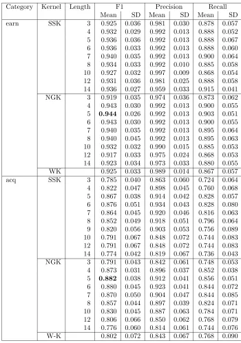
Category Kernel Length F1 Precision Recall
Mean SD Mean SD Mean SD
earn SSK 3 0.925 0.036 0.981 0.030 0.878 0.057
4 0.932 0.029 0.992 0.013 0.888 0.052 5 0.936 0.036 0.992 0.013 0.888 0.067 6 0.936 0.033 0.992 0.013 0.888 0.060 7 0.940 0.035 0.992 0.013 0.900 0.064 8 0.934 0.033 0.992 0.010 0.885 0.058 10 0.927 0.032 0.997 0.009 0.868 0.054 12 0.931 0.036 0.981 0.025 0.888 0.058 14 0.936 0.027 0.959 0.033 0.915 0.041
NGK 3 0.919 0.035 0.974 0.036 0.873 0.062
4 0.943 0.030 0.992 0.013 0.900 0.055 5 0.944 0.026 0.992 0.013 0.903 0.051 6 0.943 0.030 0.992 0.013 0.900 0.055 7 0.940 0.035 0.992 0.013 0.895 0.064 8 0.940 0.045 0.992 0.013 0.895 0.063 10 0.932 0.032 0.990 0.015 0.885 0.053 12 0.917 0.033 0.975 0.024 0.868 0.053 14 0.923 0.034 0.973 0.033 0.880 0.055
WK 0.925 0.033 0.989 0.014 0.867 0.057
acq SSK 3 0.785 0.040 0.863 0.060 0.724 0.064
4 0.822 0.047 0.898 0.045 0.760 0.068 5 0.867 0.038 0.914 0.042 0.828 0.057 6 0.876 0.051 0.934 0.043 0.828 0.080 7 0.864 0.045 0.920 0.046 0.816 0.063 8 0.852 0.049 0.918 0.051 0.796 0.064 9 0.820 0.056 0.903 0.053 0.756 0.089 10 0.791 0.067 0.848 0.072 0.744 0.083 12 0.791 0.067 0.848 0.072 0.744 0.083 14 0.774 0.042 0.819 0.067 0.736 0.043
NGK 3 0.791 0.043 0.842 0.061 0.748 0.053
4 0.873 0.031 0.896 0.037 0.852 0.038 5 0.882 0.038 0.912 0.041 0.856 0.051 6 0.880 0.045 0.923 0.041 0.844 0.072 7 0.870 0.050 0.904 0.047 0.844 0.085 8 0.857 0.044 0.897 0.039 0.824 0.071 10 0.830 0.045 0.887 0.063 0.784 0.071 12 0.806 0.066 0.850 0.062 0.768 0.079 14 0.776 0.060 0.814 0.061 0.744 0.076
[image:10.612.129.479.103.602.2]W-K 0.802 0.072 0.843 0.067 0.768 0.090
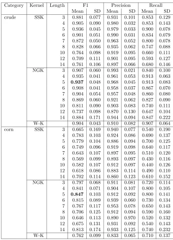
Category Kernel Length F1 Precision Recall
Mean SD Mean SD Mean SD
crude SSK 3 0.881 0.077 0.931 0.101 0.853 0.129
4 0.905 0.090 0.980 0.032 0.853 0.143 5 0.936 0.045 0.979 0.033 0.900 0.078 6 0.901 0.051 0.990 0.031 0.834 0.079 7 0.872 0.050 0.963 0.052 0.800 0.078 8 0.828 0.066 0.935 0.062 0.747 0.088 10 0.764 0.098 0.919 0.095 0.660 0.111 12 0.709 0.111 0.901 0.095 0.593 0.127 14 0.761 0.106 0.897 0.066 0.680 0.146
NGK 3 0.907 0.060 0.993 0.021 0.840 0.100
4 0.935 0.041 0.961 0.053 0.913 0.063 5 0.937 0.048 0.968 0.045 0.913 0.083 6 0.908 0.041 0.958 0.037 0.867 0.070 7 0.904 0.054 0.957 0.048 0.860 0.080 8 0.869 0.060 0.921 0.062 0.827 0.090 10 0.811 0.090 0.903 0.083 0.740 0.111 12 0.737 0.098 0.870 0.130 0.647 0.104 14 0.884 0.171 0.944 0.094 0.847 0.222
W-K 0.904 0.043 0.910 0.082 0.907 0.064
corn SSK 3 0.665 0.169 0.940 0.077 0.540 0.190
4 0.783 0.103 0.924 0.086 0.690 0.137 5 0.779 0.104 0.886 0.094 0.700 0.125 6 0.749 0.096 0.919 0.098 0.640 0.117 7 0.643 0.107 0.897 0.095 0.510 0.120 8 0.569 0.099 0.893 0.097 0.430 0.116 10 0.582 0.107 0.912 0.097 0.440 0.126 12 0.618 0.086 0.883 0.114 0.490 0.110 14 0.702 0.114 0.860 0.123 0.610 0.152
NGK 3 0.797 0.068 0.911 0.081 0.720 0.114
4 0.841 0.071 0.904 0.107 0.800 0.105 5 0.847 0.103 0.912 0.092 0.800 0.141 6 0.815 0.089 0.939 0.060 0.730 0.134 7 0.767 0.117 0.953 0.078 0.650 0.143 8 0.706 0.125 0.912 0.094 0.590 0.160 10 0.646 0.113 0.890 0.970 0.520 0.132 12 0.675 0.131 0.931 0.092 0.540 0.143 14 0.813 0.174 0.933 0.125 0.740 0.232
[image:11.612.129.480.108.595.2]W-K 0.762 0.099 0.833 0.065 0.710 0.137
adopting the experimental methodology as described. For the first set of experiments we kept the value of one parameter λ fixed and learned a classifier for different values of k. We conducted another set of experiments to observe how the performance is affected by varying the parameter λ. Finally we empirically studied the advantages of combining different kernels. This section describes the first set of experiments.
For these experiments the value of weight decay parameter was set to 0.5, and sequence length was varied. SSK was compared to NGK, where the n-grams length was also varied over a range of values. The effectiveness of SSK was also compared with the effectiveness of WK. Tables 1 and 2 describe the results of these experiments, where precision, recall and F1 numbers are shown for all three kernels. Note that these results are averaged over 10 runs of the algorithm.
From these results, we find that the performance of the classifier varies with respect to varying sequence length. SSK can be more effective for smaller or moderate substrings as compare to larger substrings. As results show, an optimal size of sequence length can be found in a region that is not very large. For each category the F1 numbers (with respect to SSK) seem to peak at a sequence length between 4 to 7. It seems that shorter or moderate contiguous substrings are able to capture the semantics better than the longer non-contiguous substrings. In practice, the size of sequence length can be set by a validation set for each category.
Tables 1 and 2 also present the results of NGK and WK. We first focus on the per-formance of an SVM classifier with NGK and compare the role of NGK with SSK for text categorization. It is interesting to note that generalisation performance of both the techniques is comparable, where NGK works on contiguous substrings and SSK works on non-contiguous substrings. The results show that the generalisation performance of an SVM classifier in conjunction with NGK is higher for short substrings and for longer substrings the performance of NGK is worse.
The classical text representation technique (WK) was also compared with SSK. It is worth noting that the performance of SSK is better that WK for each category. The size of the dataset can be one factor responsible for the degradation in the performance of WK, but these results show that SSK is an effective technique.
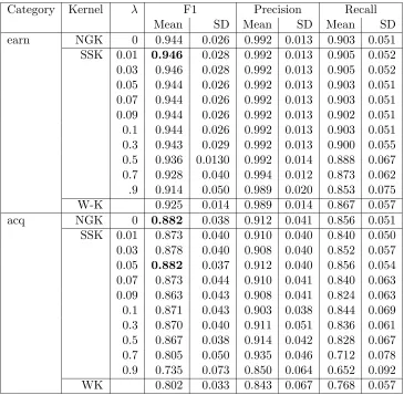
4.2 Effectiveness of Varying Weight Decay Factor
Category Kernel λ F1 Precision Recall
Mean SD Mean SD Mean SD
earn NGK 0 0.944 0.026 0.992 0.013 0.903 0.051 SSK 0.01 0.946 0.028 0.992 0.013 0.905 0.052 0.03 0.946 0.028 0.992 0.013 0.905 0.052 0.05 0.944 0.026 0.992 0.013 0.903 0.051 0.07 0.944 0.026 0.992 0.013 0.903 0.051 0.09 0.944 0.026 0.992 0.013 0.902 0.051 0.1 0.944 0.026 0.992 0.013 0.903 0.051 0.3 0.943 0.029 0.992 0.013 0.900 0.055 0.5 0.936 0.0130 0.992 0.014 0.888 0.067 0.7 0.928 0.040 0.994 0.012 0.873 0.062 .9 0.914 0.050 0.989 0.020 0.853 0.075 W-K 0.925 0.014 0.989 0.014 0.867 0.057
acq NGK 0 0.882 0.038 0.912 0.041 0.856 0.051
[image:13.612.124.489.174.531.2]SSK 0.01 0.873 0.040 0.910 0.040 0.840 0.050 0.03 0.878 0.040 0.908 0.040 0.852 0.057 0.05 0.882 0.037 0.912 0.040 0.856 0.054 0.07 0.873 0.044 0.910 0.041 0.840 0.063 0.09 0.863 0.043 0.908 0.041 0.824 0.063 0.1 0.871 0.043 0.903 0.038 0.844 0.069 0.3 0.870 0.040 0.911 0.051 0.836 0.061 0.5 0.867 0.038 0.914 0.042 0.828 0.067 0.7 0.805 0.050 0.935 0.046 0.712 0.078 0.9 0.735 0.073 0.850 0.064 0.652 0.092 WK 0.802 0.033 0.843 0.067 0.768 0.057
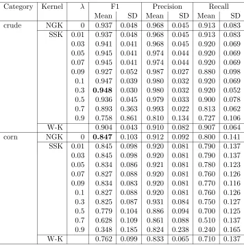
Category Kernel λ F1 Precision Recall
Mean SD Mean SD Mean SD
[image:14.612.128.484.173.531.2]crude NGK 0 0.937 0.048 0.968 0.045 0.913 0.083 SSK 0.01 0.937 0.048 0.968 0.045 0.913 0.083 0.03 0.941 0.041 0.968 0.045 0.920 0.069 0.05 0.945 0.041 0.974 0.044 0.920 0.069 0.07 0.945 0.041 0.974 0.044 0.920 0.069 0.09 0.927 0.052 0.987 0.027 0.880 0.098 0.1 0.947 0.039 0.980 0.032 0.920 0.069 0.3 0.948 0.030 0.980 0.032 0.920 0.052 0.5 0.936 0.045 0.979 0.033 0.900 0.078 0.7 0.893 0.363 0.993 0.022 0.813 0.062 0.9 0.758 0.861 0.810 0.134 0.727 0.106 W-K 0.904 0.043 0.910 0.082 0.907 0.064 corn NGK 0 0.847 0.103 0.912 0.092 0.800 0.141 SSK 0.01 0.845 0.098 0.920 0.081 0.790 0.137 0.03 0.845 0.098 0.920 0.081 0.790 0.137 0.05 0.834 0.086 0.921 0.081 0.780 0.123 0.07 0.827 0.088 0.920 0.081 0.760 0.126 0.09 0.834 0.083 0.920 0.081 0.770 0.116 0.1 0.827 0.088 0.920 0.081 0.760 0.126 0.3 0.825 0.087 0.931 0.084 0.750 0.127 0.5 0.779 0.104 0.886 0.094 0.700 0.125 0.7 0.628 0.109 0.861 0.088 0.510 0.137 0.9 0.348 0.185 0.824 0.238 0.240 0.165 W-K 0.762 0.099 0.833 0.065 0.710 0.137
of F1 at different lengths. However, the main objective of the experiments described in this section was to analyse the behaviour of SSK by varyingλ.
It is interesting to note that precision peaks at a higher value (λ = 0.7) for all the categories except one (corn). For corn the peak is achieved atλ= 0.3 and note that once a category has achieved maximum value, further increase in value of λ can degrade the effectiveness of a system substantially. Furthermore, the gain in precision is substantial for most of the categories. The gain in recall is not obtained at higher values of λ, peak is obtained at low value (λ= 0.03) for all categories except one that achieves a peak at a slightly higher value (λ= 0.05). We also note that for higher values ofλthere is substantial loss in recall. We now briefly analyse the improvement in F1 numbers, with varying λ. It seems that F1 numbers reach a maximum at a value (that is not very high) and then falls to minimum at the highest value of λ.
Polysemy is a characteristic of the English language. It seems that the technique SSK deals with this problem, as SSK returns a high similarity score if the documents share more non-contiguous substrings. A text-categorization system based on SSK can correctly classify the document that share same but semantically different words. This phenomenon is evident from the results.
We now compare the performance of SSK with other techniques. Note that the length of n-grams was set to 5 for this comparison. The results show that the effectiveness of an SVM classifier in conjunction with SSK is as good as the generalisation performance of an SVM classifier in conjunction with NGK. The results also show that the performance of SSK can be better than NGK for some cases, though the gain in performance does not seem substantial. It is worth noting that the SSK is able to achieve higher values of precision when compared to NGK.
4.3 Effectiveness of Combining Kernels
As in the preceding sections, here we describe a series of experiments to study the choice of a kernel. We observe the influence of combining kernels on generalisation performance of an SVM classifier. In other words, we empirically study the effect of adding respective inner products for different subsequence lengths and weights. Text collection and evaluation measures remain the same for these experiments.
Combining Kernels of Different Lengths
The first set of experiments considered a kernel matrix with the entries the sum of the respective entries of string subsequence kernels of different lengths. More Formally
K =¡
K(di, dj)
¢
1≤i,j≤n=
¡
K1(di, dj
¢
+K2(di, dj)
¢
1≤i,j≤n=K1 +K2
Category k1 k2 F1 Precision Recall
Mean SD Mean SD Mean SD
[image:16.612.143.471.154.569.2]earn 3 0 0.925 0.036 0.981 0.030 0.878 0.057 4 0 0.932 0.029 0.992 0.013 0.888 0.052 5 0 0.936 0.036 0.992 0.013 0.888 0.067 6 0 0.936 0.033 0.992 0.013 0.888 0.060 3 4 0.935 0.029 0.981 0.024 0.895 0.052 4 5 0.937 0.030 0.992 0.013 0.890 0.056 5 6 0.938 0.034 0.992 0.013 0.893 0.062 acq 3 0 0.785 0.040 0.863 0.060 0.724 0.064 4 0 0.822 0.047 0.898 0.045 0.760 0.068 5 0 0.867 0.038 0.914 0.042 0.828 0.057 6 0 0.876 0.051 0.934 0.043 0.828 0.080 3 4 0.827 0.028 0.866 0.034 0.792 0.037 4 5 0.857 0.036 0.918 0.027 0.804 0.051 5 6 0.866 0.044 0.925 0.043 0.816 0.066 crude 3 0 0.881 0.077 0.931 0.101 0.853 0.129 4 0 0.905 0.090 0.980 0.032 0.853 0.143 5 0 0.936 0.045 0.979 0.033 0.900 0.078 6 0 0.901 0.051 0.990 0.031 0.834 0.079 3 4 0.932 0.048 0.958 0.071 0.913 0.070 4 5 0.936 0.049 0.981 0.042 0.90 0.090 5 6 0.916 0.062 0.986 0.03 0.86 0.101 corn 3 0 0.665 0.169 0.940 0.077 0.540 0.190 4 0 0.783 0.103 0.924 0.086 0.690 0.137 5 0 0.779 0.104 0.886 0.094 0.700 0.125 6 0 0.749 0.096 0.919 0.098 0.640 0.117 3 4 0.769 0.080 0.904 0.092 0.680 0.113 4 5 0.776 0.090 0.904 0.093 0.69 0.120 5 6 0.761 0.080 0.908 0.088 0.660 0.966
the combination of kernels appears of no gain showing that both the kernels give similar information. Note that all the results presented in this section are averaged over 10 samples of the data.
Combining NGK and SSK
We now present the experiments by adding the respective entries in a string subsequence kernel matrix and an n-grams kernel matrix. We set the length for both the kernels to 5, and for SSK the value of λwas set to 0.5. The results of this set of experiments are shown in Table 6. We not only combined the SSK and NGK but we also observed the influence of combining weighted entries of respective kernel matrices. The entries of NGK were weighted more as compare to SSK, formally
K=wngN GK+wskSSK.
Unfortunately this set of experiments does not yield any improvement in the generalisation performance of an SVM classifier.
Combining SSK with different λ’s
Another set of experiments was conducted to evaluate the effect of combining SSK for different λ’s. The results are reported in Table 7. The length of the subsequence was set to 5 and two values (0.05 and 0.5)of λ were combined. The results showed that this methodology of adding respective entries of string subsequence kernels for differentλ’s and using the resultant kernel matrix with an SVM does not improve the performance of the system substantially.
5. Approximating Kernels
When constructing a Gram matrix, the computational cost is often high. This may be due to either the need for a large number of kernel evaluations (i.e. there is a large training set) or due to the high computational cost of evaluating the kernel itself. In some circumstances, both points may be true.
The approximation approach we adopt is based on a more general empirical kernel map introduced by Sch¨olkopf et al. (1999). We consider the special case when the set of vectors is chosen to be orthogonal. Assume we have some training points (xi, yi) ∈ X×Y, and
some kernel function K(x, z) corresponding to a feature space mapping φ : X 7→ F such thatK(x, z) =hφ(x), φ(z)i. Consider a set S of vectorsS ={si ∈ X }. If the cardinality of
S is equal to the dimensionality of the space F and the vectors φ(si) are orthogonal (i.e.
K(si, sj) =Cδij)1, then the following is true:
K(x, z) = 1 C
X
si∈S
K(x, si)K(z, si). (3)
Category wng wsk F1 Precision Recall
Mean SD Mean SD Mean SD
earn 1 0 0.944 0.026 0.992 0.013 0.903 0.051 0 1 0.936 0.013 0.992 0.014 0.888 0.067 0.5 0.5 0.944 0.026 0.992 0.013 0.903 0.051 0.6 0.4 0.941 0.029 0.992 0.013 0.898 0.055 0.7 0.3 0.941 0.029 0.992 0.013 0.898 0.055 0.8 0.2 0.944 0.030 0.992 0.013 0.903 0.060 0.9 0.1 0.943 0.0260 0.992 0.013 0.900 0.050
acq 1 0 0.882 0.038 0.912 0.041 0.856 0.051
0 1 0.867 0.038 0.914 0.042 0.828 0.067 0.5 0.5 0.865 0.035 0.917 0.045 0.820 0.051 0.6 0.4 0.878 0.031 0.908 0.036 0.852 0.046 0.7 0.3 0.868 0.047 0.909 0.040 0.832 0.073 0.8 0.2 0.875 0.033 0.913 0.050 0.844 0.058 0.9 0.1 0.875 0.040 0.910 0.040 0.844 0.058 crude 1 1 0.937 0.048 0.968 0.045 0.913 0.083 0 1 0.936 0.045 0.979 0.033 0.900 0.078 0.5 0.5 0.940 0.0360 0.987 0.027 0.900 0.072 0.6 0.4 0.937 0.040 0.980 0.032 0.900 0.072 0.7 0.3 0.934 0.057 0.994 0.020 0.887 0.105 0.8 0.2 0.928 0.057 0.981 0.042 0.887 0.104 0.9 0.1 0.926 0.063 1.000 0.000 0.867 0.104 corn 1 0 0.847 0.103 0.912 0.092 0.800 0.141 0 1 0.779 0.104 0.886 0.094 0.700 0.125 0.5 0.5 0.843 0.095 0.929 0.085 0.750 0.127 0.6 0.4 0.836 0.091 0.943 0.085 0.760 0.126 0.7 0.3 0.827 0.098 0.916 0.083 0.760 0.126 0.8 0.2 0.831 0.093 0.930 0.084 0.760 0.126 0.9 0.1 0.849 0.092 0.943 0.084 0.780 0.123
Category λ’s F1 Precision Recall
1 2 Mean SD Mean SD Mean SD
[image:19.612.132.479.88.283.2]earn 0.05 0.0 0.944 0.026 0.992 0.013 0.903 0.051 0.5 0.0 0.936 0.013 0.992 0.014 0.888 0.067 .05 0.5 0.949 0.024 0.991 0.013 0.911 0.044 acq 0.05 0.0 0.882 0.037 0.912 0.040 0.856 0.054 0.5 0.0 0.867 0.038 0.914 0.042 0.828 0.067 0.05 0.5 0.869 0.041 0.921 0.042 0.824 0.063 crude 0.05 0.0 0.945 0.041 0.974 0.044 0.920 0.069 0.5 0.0 0.936 0.045 0.979 0.033 0.900 0.078 0.05 0.5 0.940 0.039 0.980 0.032 0.907 0.071 corn 0.05 0.0 0.834 0.086 0.921 0.081 0.780 0.123 0.5 0.0 0.779 0.104 0.886 0.094 0.700 0.125 0.05 0.05 0.818 0.088 0.930 0.085 0.740 0.126
Table 7: The performance (F1, precision, recall) of SVM with combined kernels for Reuters categories earn, acq, corn and crude. The SSK for different λ’s have been com-bined. The results are averaged and standard deviation is also given.
This follows from the fact thatφ(x) = C1 P
si∈SK(x, si)φ(si) andφ(z) = 1
C
P
sj∈SK(z, sj)φ(sj), so that
K(x, z) = 1
C2 X
si,sj∈S
K(x, si)K(z, sj)Cδij
= 1 C
X
si∈S
K(x, si)K(z, si).
If instead of forming a complete orthonormal basis, the cardinality of ˜S ⊆S is less than the dimensionality of X or the vectors si are not fully orthogonal, then we can construct
an approximation to the kernelK:
K(x, z)≈ X
si∈S˜
K(x, si)K(z, si). (4)
In this paper we propose to use the above fact in conjunction with an efficient method of choosing ˜S to construct a good approximation of the kernel function. If the set ˜S is carefully constructed, then the production of a Gram matrix which is closely aligned to the true Gram matrix can be achieved with a fraction of the computational cost. A problem at this stage is how to choose the set ˜Sand how to ensure that the vectorsφ(si) are orthogonal.
5.1 Choosing a subset of features
selecting the top few according to frequency. Recently the Gram-Schmidt procedure has also been applied to kernel matrices in order to choose orthogonal features (Smola and Sch¨olkopf, 2000). Other approaches may include selecting data points from the training set which are close to being orthonormal, or using a generative model to form ˜S. Whichever method is chosen, the result is a low rank approximation of the Gram matrix K. This is also the aim of techniques such as kernel principal components analysis or latent semantic kernels.
We are going to use a heuristic based on explicitly generating an orthogonal and complete set of data, and from these choosing the best points according to a given criteria, so ˜S ⊂S whereSis orthogonal and complete. Suppose that the set ˜Shas sizelwith each entry having n′ characters. In this case the evaluation of the feature vector will require O(nn′lt) for the string kernel of length nand a document of lengtht. The computation of the approximate string kernel would therefore require O(nn′lt) as compared with O(nt2) required by the direct menthod. Providedn′l < tthis will represent a saving. The improvement is greater if we evaluate a kernel matrix for a training set of sizem, documents each of lengtht. Since this requiresO(mnn′lt+lm2) as opposed toO(m2nt2) required for a direct evaluation of all the entries. In this case savings will be made ifl < nt2 and n′l < mt. We should therefore choose n′ small and control the size of l. We enforce both of these inequalities in Section 6 when using the string kernel on the Reuters data set. Before we discuss a particular implementation of this method however, we must first discuss a method of measuring the similarity of two Gram matrices.
5.2 Similarity of Gram Matrices
In order to discover how many features are needed to obtain a good approximation of the true Gram matrix, we need a measure of similarity between Gram matrices. In this paper we use the notion of alignment (Cristianini et al., to appear) which was recently proposed. In the paper the Frobenius inner product is used between Gram matrices hK1, K2iF =
Pm
i,j=1K1(xi, xj)K2(xi, xj).
The measure of alignment between two matrices is then given as follows:
Definition 3 Alignment The (empirical) alignment of a kernelk1 with a kernel k2 with
respect to the sampleS is the quantity
ˆ
A(S, k1, k2) =
hK1, K2iF
p
hK1, K1iFhK2, K2iF
,
where Ki is the kernel matrix for the sample S using kernel ki.
This is the measure which we will use here. If the matrices are fully aligned (i.e. they are the same) then the alignment measure is 1, see (Cristianini et al., to appear) or (Cristianini et al., 2001) for details of kernel alignment.
6. Approximating the string kernel
6.1 Obtaining the approximation
As mentioned above, the string kernel has time complexity of O(n|s||t|), where n is the length of sub-sequences which we are considering, and sand t are the length of the docu-ments involved. For datasets such as the Reuters data set, which contains approximately 9600 training examples and 3200 test examples with an average length of approximately 2300 characters, the string kernel is too expensive to apply on large text collections.
Our heuristic for obtaining the set ˜S is as follows:
1. We choose a substring size n.
2. We enumerate all possible contiguous strings of lengthn.
3. We choose the x strings of length n which occur most frequently in the dataset and this forms our set ˜S.
Notice that by definitionall such strings of length nare orthogonal (i.e. K(si, sj) = (Cδij)
for some constantC when used in conjunction with the string kernel of degree n. Using all features is therefore exactly equivalent to the string kernel, whereas using a subset gives an approximation. This is far quicker than calculating the dot product between documents. We would expect the most frequent features to result in a good approximation of the kernel, as we are discarding the less informative features. It is possible that some of the frequent features may be non-informative however, and a possibility for improving this naive approach would be to use mutual information as part of the selection process.
6.2 Selecting the subset
1000 2000 3000 4000 5000 6000 7000 8000 9000 10000 0.5
0.6 0.7 0.8 0.9 1
[image:22.612.179.429.92.290.2]Frequent Infrequent Random
Figure 1: Alignment scores (against the Gram matrix generated by the full string kernel) when using the most frequent, infrequent and random selection of features.
string kernel. The full Gram matrices for large datasets can now be efficiently generated and used with any kernel algorithm.
7. Experimental Results
In order to evaluate the proposed approach we conducted experiments based on the “ModApte” split of the Reuters-21578 dataset. The only pre-processing run on the dataset before ex-perimentation was the removal of common stop-words. We ran an approximation of the string kernel withk= 3,4,5 on the full Reuters data set. In order to compare our results to current techniques, we used a bag of words approach. We also used the softwareSV Mlight
(Joachims, 1999) to run the experiments once the bag of words and approximation features had been generated. Performance of the proposed technique was compared withn-grams. Forn-grams as pre-processing the stop words were removed. We conducted experiments for n= 3,4,5. Note that for all the experiments described in this section we used theSV Mlight
1000 3000 earn 0.97 0.97 acq 0.88 0.85 ship 0.10 0.53 corn 0.15 0.65
Table 8: F1 numbers for 4 Reuters categories. Comparing different numbers of features in the approximation to the SSK on 4 categories of the Reuters dataset.
Category WK NGK Approximated SSK
n k
3 4 5 3 4 5
earn 0.982 0.982 0.984 0.974 0.970 0.970 0.970 acq 0.948 0.919 0.932 0.887 0.850 0.880 0.880 money-fx 0.775 0.744 0.757 0.692 0.700 0.760 0.740 grain 0.930 0.852 0.840 0.758 0.800 0.820 0.800 crude 0.880 0.857 0.848 0.640 0.820 0.840 0.840 trade 0.761 0.774 0.779 0.767 0.700 0.730 0.730 interest 0.691 0.708 0.719 0.503 0.630 0.660 0.690 ship 0.797 0.657 0.626 0.321 0.610 0.650 0.530 wheat 0.870 0.803 0.797 0.629 0.780 0.790 0.820 corn 0.895 0.761 0.610 0.459 0.630 0.630 0.680
Table 9: F1 numbers for SVM with WK, NGK and SSK for top-ten Reuters categories.
comparable to WK and NGK. In order to gauge the efficiency of the approach, remember that the string kernel takes O(n|s||t|) time. Using n= 5 and an approximate word length of 2000 characters, with a training set of 9603 documents (as in the Reuters dataset) this number becomes 9603×9603×5×2000×2000≈1.8x10¹⁵ to naively generate the Gram matrix. For the approximation approach however, using 100 features (i.e. strings of length 3) we have 9603×100×5×3×2000≈2.8x10¹⁰ which is considerably faster.
8. Conclusions
The paper has presented a novel kernel and its approximation for text analysis. The per-formance of the string subsequence kernel was empirically tested by applying it to a text categorization task. This kernel can be used with any kernel-based learning system, for example in clustering, categorization, ranking, etc. In this paper we have focused on text categorization, using a Support Vector Machine.
[image:23.612.148.464.225.406.2]This paper builds on preliminary results presented in Lodhi et al. (2001). This is most likely due to the extreme computational cost of accessing such a feature space without using the kernel trick. For a given sequence length k the features are indexed by all strings of length k. Direct computation of all the relevant features would be impractical even for moderately sized texts andk. We have used a dynamic programming style computation for computing the kernel directly from the input sequences without explicitly calculating the feature vectors. This has been possible since we have used a kernel-based learning machine. The experiments indicate that our algorithm can provide an effective alternative to the more standard word feature based kernel used in previous SVM applications for text classification (Joachims, 1998). We were also able to compare them with results obtained using a string kernel that only considered contiguous strings, thus providing a continuum of varying the parameterλto 0. The kernel for contiguous strings was also combined with the non-contiguous kernel to examine to what extent different features were being used in the classification.
In addition different lengths of strings were considered and a comparison made of the results obtained on Reuters data using a range of different values.
In order to apply the proposed approach on large datasets, we derived a fast algo-rithm that approximates the exact string kernel. We have also introduced a method for approximating kernels based on using a subset of orthogonal features. This allows the fast construction of kernel Gram matrices. We have shown that by using all features we arrive exactly at the string kernel solution, however we have also shown that good approximations can be obtained by using a relatively small number of features. In order to illustrate this technique we conducted an extensive set of experiments. We provided experimental results using the string kernel which is known to be computationally expensive. Using the approx-imation however, we were able to achieve results on the full Reuters dataset which were comparable to those produced by the bag of words approach.
The results on the full Reuters dataset were, however, less encouraging. In most cases the word kernel and contiguousn-grams kernel outperformed the string kernel. This led us to conjecture that the excellent results on smaller datasets demonstrate that the kernel is performing something similar to stemming, hence providing semantic links between words that the word kernel must view as distinct. This effect is no longer so important in large datasets where there is enough data to learn the relevance of the terms.
It is an open question to see whether ranking the features according to positive and negative examples and introducing a weighting scheme will improve results. Also once a good approximation to the Gram matrix is produced, it can easily be used with other kernel methods (e.g. for clustering, principal components analysis, etc.). The relationship between the quality of the approximation and the generalisation error achieved by an algorithm also needs to be explored. One could also consider using the fast approximation with very few features to obtain a very coarse Gram matrix. A preliminary estimate of the support vectors could then be obtained, and the entries for these vectors could then be refined. This could give rise to a fast form of chunking for large datasets.
the extension of the techniques to strings of syllables and words as well as to types of data other than text.
References
B. E. Boser, I. M. Guyon, and V. N. Vapnik. A training algorithm for optimal margin classifiers. In D. Haussler, editor, Proceedings of the 5th Annual ACM Workshop on Computational Learning Theory, pages 144–152, Pittsburgh, PA, July 1992. ACM Press.
W. B. Cavnar. Using an n-gram based document representation with a vec-tor processing retrieval model. In D. K. Harman, editor, Proceedings of
TREC –3, 3rd Text Retrieval Conference, pages 269–278, Gaithersburg,
Mary-land, US, 1994. National Institute of Standards and Technology, Gaithersburg, US. http://trec.nist.gov/pubs/trec3/t3proceedings.html.
N. Cristianini, A. Elisseef, and J. Shawe-Taylor. On optimizing kernel alignment. Technical Report NC-TR-01-087, Royal Holloway, University of London, UK, 2001.
N. Cristianini, A. Elisseef, and J. Shawe-Taylor. On kernel-target alignment. In Neural Information Processing System (NIPS ’01), to appear.
N. Cristianini and J. Shawe-Taylor.An introduction to Support Vector Machines. Cambridge University Press, Cambridge, UK, 2000.
T. Friess, N. Cristianini, and C. Campbell. The kernel-adatron: a fast and simple training procedure for support vector machines. In J. Shavlik, editor, Proceedings of the 15th International Conference on Machine Learning. Morgan Kaufmann, 1998.
D. Haussler. Convolution kernels on discrete structures. Technical Report UCSC-CRL-99-10, University of California in Santa Cruz, Computer Science Department, July 1999.
S. Huffman. Acquaintance: Language-independent document categorization by n-grams. In D. K. Harman and E. M. Voorhees, editors, Proceedings of
TREC –4, 4th Text Retrieval Conference, pages 359–371, Gaithersburg,
Mary-land, US, 1995. National Institute of Standards and Technology, Gaithersburg, US. http://trec.nist.gov/pubs/trec4/t3proceedings.html.
T. Joachims. Text categorization with support vector machines: Learning with many rele-vant features. In Claire N´edellec and C´eline Rouveirol, editors, Proceedings of the Euro-pean Conference on Machine Learning, pages 137–142, Berlin, 1998. Springer.
T. Joachims. Making large–scale SVM learning practical. In B. Sch¨olkopf, C. J. C. Burges, and A. J. Smola, editors,Advances in Kernel Methods — Support Vector Learning, pages 169–184, Cambridge, MA, 1999. MIT Press.
J. Mercer. Functions of positive and negative type and their connection with the theory of integral equations. Philosophical Transactions of the Royal Society London (A), 209: 415–446, 1909.
G. Salton, A. Wong, and C. Yang. A vector space model for automatic indexing. Commu-nications of the ACM, 18(11):613–620, 1975.
B. Sch¨olkopf. Support Vector Learning. R. Oldenbourg Verlag, M¨unchen, 1997. Doktorarbeit, Technische Universit¨at Berlin. Available from http://www.kyb.tuebingen.mpg.de/∼bs.
B. Sch¨olkopf, S. Mika, C. Burges, P. Knirsch, K.-R.M¨uller, G. R¨atsch, and A. Smola. Input space vs. feature space in kernel-based methods. IEEE Transactions on Neural Networks, 10(5):1000–1017, 1999.
A. J. Smola and B. Sch¨olkopf. Sparse greedy matrix approximation for machine learning. In P. Langley, editor, Proceedings of the Seventeenth International Conference on Machine Learning, pages 911–918. Morgan-Kauffman, 2000.
V. Vapnik. The Nature of Statistical Learning Theory. Springer Verlag, New York, 1995.
C. Watkins. Dynamic alignment kernels. In A. J. Smola, P. L. Bartlett, B. Sch¨olkopf, and D. Schuurmans, editors, Advances in Large Margin Classifiers, pages 39–50, Cambridge, MA, 2000. MIT Press.