Asymptotic Bayesian Decision Feedback Equalizer
Using a Set of Hyperplanes
Sheng Chen, Senior Member, IEEE, Bernard Mulgrew, Member, IEEE, and Lajos Hanzo
Abstract—We present a signal space partitioning technique for
realizing the optimal Bayesian decision feedback equalizer (DFE). It is known that when the signal-to-noise ratio (SNR) tends to in-finity, the decision boundary of the Bayesian DFE is asymptotically piecewise linear and consists of several hyperplanes. The proposed technique determines these hyperplanes explicitly and uses them to partition the observation signal space. The resulting equalizer is made up of a set of parallel linear discriminant functions and a Boolean mapper. Unlike the existing signal space partitioning technique of Kim and Moon, which involves complex combina-torial search and optimization in design, our design procedure is simple and straightforward, and guarantees to achieve the asymp-totic Bayesian DFE.
Index Terms—Asymptotic decision boundary, Bayesian decision
feedback equalizer, signal space partition.
I. INTRODUCTION
E
QUALIZATION technique plays an ever-increasing role in combating distortion and interference in communica-tion links [1], [2] and high-density data storage systems [3], [4]. The equalization topic is well researched, and a variety of solutions are available. The maximum a posteriori probability (MAP) sequence detector [5]–[7], although providing the lowest bit error rate (BER) attainable, finds little application in prac-tice due to it computational complexity. The more popular se-quence detector is the maximum likelihood sese-quence estima-tion (MLSE) based on teh Viterbi algorithm [8], which is still computationally expensive and requires a sufficiently long de-cision delay to guarantee the optimal or near optimal perfor-mance. Many practical techniques employ a symbol-decision finite-memory structure with a fixed delay and are based on adaptive linear filter algorithms [1] with very low complexity. In particular, the conventional or linear-combiner DFE offers acceptable performance in many practical situations.The BER gap between the MLSE and the conventional DFE for practical SNR conditions is large, and recent research in neural network equalizers [9]–[15] has attempted to fill in this gap and to strike a good balance between performance and com-plexity. A discussion on why it is worth considering the appli-cation of neural networks to equalization is given in [16]. It
Manuscript received July 7, 1999; revised July 20, 2000. The associate editor coordinating the review of this paper and approving it for publication was Dr. Vikram Krishnamurthy.
S. Chen and L. Hanzo are with Department of Electronics and Computer Sci-ence, University of Southampton, U.K. (e-mail: [email protected]; www-mobile.ecs.soton.ac.uk).
B. Mulgrew is with Department of Electronics and Electrical Engineering, University of Edinburgh, Edinburgh, U.K.
Publisher Item Identifier S 1053-587X(00)10164-3.
is well known that the optimal solution for the symbol-deci-sion finite-memory equalizer structure with a fixed delay is the Bayesian DFE [11], [17], and this equalization solution has an equivalent form to a radial basis function network. The compu-tational complexity of the Bayesian DFE is, however, consider-ably more than that of the simple linear-combiner DFE. Various neural network equalizers can be regarded as realizations or ap-proximations of this Bayesian solution with various degrees of complexity.
Geometrically, the conventional DFE partitions the observa-tion space with a hyperplane. The optimal Bayesian decision boundary, however, is a hypersurface in the observation space [11]. It can be shown that asymptotically, as the SNR tends to in-finity, the Bayesian hypersurface becomes piecewise linear and is made up of a set of hyperplanes [18]. In practice, at large rather than infinite SNR, the performance difference between Bayesian decision boundary and a piecewise linear approxima-tion is negligible. This motivates research using multiple hyper-planes to partition the signal space. Kim and Moon [19], [20] re-cently developed a signal space partitioning technique for equal-ization. This technique basically determines a set of hyperplanes that separate clusters of noiseless channel states or signals. A combinatorial search and optimization process is carried out to find these hyperplanes, which requires extensive computational efforts. The convex regions associated with individual channel states are constructed by appropriately intersecting hyperplanes. The overall decision region is then formed from these convex re-gions.
Kim and Moon’s design method results in an equalizer structure consisting of parallel linear discriminant functions and a many-to-one Boolean mapper. The decision complexity and performance of the detector are controlled during design by a specified minimum separating distance. Although it is possible to achieve the asymptotic Bayesian solution by an appropriate choice of the minimum separating distance, this is by no means guaranteed as the combinatorial search and optimization process does not necessarily produce the set of hyperplanes that form the asymptotic Bayesian decision boundary.
In this paper, we propose a much simpler alternative design. Specifically, the set of hyperplanes that form the asymp-totic Bayesian decision boundary can straightforwardly be determined, thus avoiding the design complexity of Kim and Moon’s method. Furthermore, our design guarantees to achieve, asymptotically, the optimal Bayesian solution. The decision complexity of the detector is solely determined by the channel geometric structure. Section II reviews the Bayesian DFE, which also serves to introduce the necessary notations
and definitions. The proposed new signal space partitioning technique is presented in Section III. Simulation results are provided in Section IV, and concluding remarks are given in Section V.
II. BAYESIANDECISIONFEEDBACKEQUALIZER
We will assume that the channel is modeled as a finite impulse response filter with an additive noise source. Specifically, the received signal at sample is
(1)
where
noiseless channel observation; channel length;
channel tap weights;
Gaussian white noise sequence having zero mean and variance ;
independently identically distributed symbol se-quence and is uncorrelated with .
The SNR of the system is defined as
SNR (2)
where is the symbol variance. In this study, for the purpose of easy geometrical visualization, we will assume that the channel is real-valued and that the transmitted symbol is binary, taking value from the set . There is no difficulty, however, to apply the current results to complex-valued channels and mul-tilevel signaling schemes.
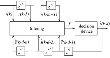
The structure of a generic DFE is depicted in Fig. 1. The equalization process defined in Fig. 1 uses the information present in the channel observation vector
(3)
and the past detected symbol vector
(4)
to produce an estimate of , where the integers , , and are the decision delay and the feedforward and feedback orders, respectively. Without the loss of generality, we
will choose , and as this choice of
the DFE structure parameters is sufficient to guarantee the linear separability (see Proposition 1 in this section). The observation vector (3) can be arranged as
(5)
where ,
with
(6)
and the channel impulse response matrix has the form
(7)
with the matrix and matrix defined by
. .. ...
..
. . .. . ..
(8)
and
. .. ... . ..
..
. . .. . ..
(9)
Past decisions on the symbols , are
used to cancel intersymbol interference terms from observation samples. In this process, past decisions ,
are assumed to be correct. Under this assumption, , and
(10)
Thus, the decision feedback can be viewed as a translation of the original space into a new space :
(11)
Let be the unit delay operator. The elements of can be computed recursively according to
(12)
The DFE structure of Fig. 1 is therefore equivalent to the equal-ization structure of Fig. 2.
Let the sequences or states of be ,
. Define the set of the noiseless channel states in the translated space by
(13)
This set can be partitioned into two subsets conditioned on :
(14)
We have the following linear separability property.
Proposition 1: and are linearly separable. The proof is straightforward. Choose the weights of a
hyper-plane to be
Fig. 1. Generic decision feedback equalizer.f is the decision variable.
Fig. 2. Translated decision feedback equalizer.f is the decision variable.
For any and , we have
and .
Proposition 1 states a well-known fact that it is always possible to construct a single hyperplane to correctly sepa-rate opposite-class channel states. What is interesting is that the weight vector (15) is the limit of the minimum mean square error (MMSE) solution for the conventional DFE with SNR [21]. This implies that the MMSE solution does not achieve the full performance potential of the linear-combiner DFE. How to construct a single optimal hyperplane to realize the minimum BER linear-combiner DFE has been addressed in [21] and [22].
The true optimal solution for the equalization structure of Fig. 2, however, cannot be realized using a single hyperplane. Assuming equiprobable channel states, the optimal solution for the equalization structure of Fig. 2 is given by the following Bayesian decision function [11], [15]:
(16)
with the minimum-error-probability decision defined by
. (17)
The decision boundary of this Bayesian DFE
(18)
is generally a hypersurface. Before describing the asymptotic Bayesian decision boundary for SNR (or ), we introduce the following definition.
Definition 1: A pair of opposite-class states is
said to be dominant if , , :
(19)
where
(20)
Proposition 2: Asymptotically, the decision boundary
is piecewise linear and made up of a set of hyperplanes. Each of these hyperplanes is defined by a pair of dominant channel states, and the hyperplane is orthogonal to the line connecting the pair of dominant states and passes through the midpoint of the line.
Proof: Consider . As , Iltis [18] has
shown that a necessary condition for a point is
(21)
where denotes an arbitrary vector in the subspace orthogonal to , , and are a pair of dominant states; the sufficient
conditions for are
(22)
(23)
(24)
Proposition 2 follows as a direct consequence.
Remark 1: The section of the decision boundary within the “influencing domain” of a dominant pair , as de-fined by (22) and (23), is a section of the hyperplane that passes through the midpoint of the line connecting the pair, as indicated in (21) and (24). Although the boundary described in Proposi-tion 2 is only exact in the limit case of infinite SNR, our empir-ical experience, and others such as [18], have shown that for the SNRs on the order of 10–20 dB, the true Bayesian boundary is closely approximated by the asymptotic multiple hyperplane form, and the two forms are often indistinguishable.
Remark 2: It should be emphasized that the pairs
needed to define the boundary hyperplanes are only a subset of all the possible signal states . For the
generic channel , it is impossible to
determine a theoretic bound for the number of the dominant pairs . Empirically, we have found that usually,
[image:3.612.303.548.392.493.2]Fig. 3. Two typical cases of the asymptotic Bayesian decision boundary for channela = [a ; a ] .
III. ASYMPTOTICBAYESIANDFE USINGHYPERPLANES
In a previous work [23], the Bayesian solution is approxi-mated by only using the set of dominant state pairs, which de-termine the asymptotic Bayesian decision boundary, in the com-putation of the Bayesian decision variable (16). In this study, we consider using the multiple-hyperplane detector structure of Kim and Moon [19], [20] (see Fig. 4) to realize the asymptotic Bayesian DFE. Our design procedure for constructing the de-tector, which is very different from that of Kim and Moon, is as follows:
Step 1) Select all pairs of dominant channel states from the state set . For each pair, compute a hyperplane that separates these two opposite-class states. Step 2) A Boolean logic function is obtained to make a final
decision based on the location of the observation vector relative to each hyperplane. This is achieved by first defining a convex region associated with each state in a given class and then forming a union of these regions.
From the proof of Proposition 2, it is easily seen that pairs of dominant states that define the asymptotic boundary can be selected using the following algorithm:
L = 0; FOR
FOR
; ;
IF AND
;
; END IF
NEXT NEXT
Fig. 4. Asymptotic Bayesian DFE using a set of hyperplanes.
Each pair determines a hyperplane
(25)
that is a part of the asymptotic Bayesian decision boundary. The weight vector and bias of the hyperplane can be computed straightforwardly as
(26)
and
(27)
Notice that we have applied the theory of support vector ma-chines [22], [24], [25] in determining the hyperplane with as its two support vectors. That is, the hyperplane defined by (26) and (27) is a canonical hyperplane [24] having
the property and . Let us
intro-duce the definition of sufficient separability.
Definition 2: A state is said to be sufficiently
sepa-rable by the hyperplane if can separate correctly with
a “canonical distance” .
Notice that is sufficiently separable by if and
only if . Similarly, is sufficiently
separable by if and only if . All the states in are tested to see they can be separated sufficiently by ,
. This generates the following matrix:
..
. ... ... ... ... ...
where , , and states are numbered
such that for and for
. The rule in generating this matrix is as follows: If can sufficiently be separated by , ; otherwise, . Notice that in every row, there are at least two nonzero elements (associated with a dominant pair), and in every column, there is at least one nonzero element.
The half-space defined by a hyperplane is
[image:4.612.89.244.61.253.2]To construct a convex region corresponding to a state , select those hyperplanes that can sufficiently sep-arate and denote
(29)
Then, is obtained by the intersection of all the with
(30)
In fact, it may not be necessary to use every hyperplanes defined in to construct . A subset of these hyperplanes will be enough in the construction of , provided that every state in can sufficiently be separated by at least one hyperplane in the subset. The overall decision region associated with the decision is simply formed as the union of all the
(31)
For an illustration, consider Fig. 3(b). It is easily seen
that , , , and
. Thus, , and .
The complete matrix of the separating hyperplanes and channel states is given in Table I. From Table I, it can be seen that the state requires two hyperplanes and to be separated from the states in . The region for is the intersection of the two half spaces and defined by and . The hyperplane can separate from the states in . The region for is thus the half-space defined by . The overall decision region is the
union of and .
The Boolean logic function for the detector depicted in Fig. 4 is now completely defined. Let a threshold detector output for a linear discriminant function
have Boolean logic value 1 or 0 depending on
or not. A Boolean logic value indicating whether or not is obtained via a logic AND operation
of : . A Boolean logic value indicating
whether [that is, ] or not is obtained
via a logicORoperation of for all . This detector achieves, asymptotically, the optimal Bayesian performance since it realizes exactly the asymptotic Bayesian decision boundary.
In our design, the determination of appropriate multiple hyperplanes for the observation space partitioning is straight-forward. The required number of hyperplanes is specified by the asymptotic Bayesian decision boundary and, therefore, is defined by the channel impulse response. The algorithm automatically selects the set of hyperplanes, which specify the asymptotic Bayesian decision boundary, with very low computational efforts in this design stage. This should be compared with Kim and Moon’s signal space partitioning technique [19], [20]. For purposes of comparison, their design
TABLE I
MATRIX OFSEPERATINGHYPERPLANES ANDCHANNELSTATES FORTHE
EXAMPLEGIVEN INFIG. 3(b)
TABLE II
COMPARISON OFDECISIONCOMPLEXITY FORTHECONVENTIONALDFE, FULL
BAYESIAN,ANDOURMULTIPLE-HYPERPLANEDETECTORS.L (USUALLY
2 ) IS THENUMBER OFHYPERPLANES,ANDn IS THELENGTH OF
CHANNELIMPULSERESPONSE. THEDFE STRUCTUREISCHOSEN TOBE
m = n , d = n 0 1,ANDn = n 0 1
procedure is summarized in the Appendix, where it can be seen that a combinatorial search process with nonlinear gradient optimization and integer programming is performed to find a set of separating hyperplanes, given a specified minimum distance. Their design procedure therefore requires extensive computation. Furthermore, their procedure is not guaranteed to converge to the infinite-SNR asymptote of the optimal Bayesian detector. The performance of their detector will generally lie between the conventional DFE and the asymptotic Bayesian DFE, depending on the specified minimum distance in the design.
Table II compares decision complexity for the conventional DFE, the full Bayesian DFE, and our multiple-hyperplane de-tector. The conventional DFE has the lowest complexity as it is made up of a single hyperplane. Our detector generally has much simpler decision complexity than the full Bayesian de-tector since usually, . Obviously, the decision com-plexity of Kim and Moon’s multiple-hyperplane detector can be similar to the conventional DFE or similar to or higher than our detector, depending on the actual number of hyperplanes se-lected in the design.
IV. SIMULATIONRESULTS
Two channels were used to demonstrate the proposed new signal space partitioning technique. The BER performance of the multiple-hyperplane detector was compared with those of the full Bayesian DFE and the conventional MMSE DFE. Ex-cept otherwise explicitly stated, all the BER results were ob-tained with detected symbols being fed back.
Channel A: The impulse response was specified by
(32)
The structure parameters of the DFE were accordingly set to
, , and . The channel state set had
states , and therefore, the convex region for is the intersection of the two half spaces and . The states and are separated from by the two hy-perplanes and . Thus, is the intersection of the half spaces and . The state is separated by the single hyperplane from all the opposite-class states, and the convex region for is the half-space defined by . The overall decision region is the union of ,
, and .
The resulting detector requires 15 multiplications and 15 ad-ditions to detect a symbol, compared with 32 multiplications, 47 additions, and eight evaluations required by the full Bayesian detector and only three multiplications and two addi-tions required by the conventional DFE. The BERs of this mul-tiple-hyperplane detector are compared with those of the full Bayesian DFE in Fig. 5 under different SNR conditions. It can be seen from Fig. 5 that there is hardly any BER performance difference between the two equalizers. The BER curve of the conventional MMSE DFE is also depicted in Fig. 5.
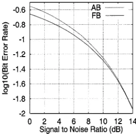
Channel B: Channel B had an impulse response given by
(33)
The DFE structure was defined by , , and . The state set had 16 states. The asymptotic Bayesian decision boundary in this case consisted of seven hyperplanes, and they were automatically selected by the algorithm. The matrix of the separating hyperplanes and channel states is given in Table IV. The states , , , and require only the hyperplane to separate them from all the opposite-class states. Thus,
, , , and are defined by the half-space specified by . As the states and are separated from
by the two hyperplanes and , is the
intersection of the two half-spaces and . The state requires the two hyperplanes and to separate it from all the opposite-class states, and the convex region is thus the intersection of and . Similarly, the convex region for is the intersection of and . The overall decision region is the union of the four convex regions
, , , and .
This multiple-hyperplane-based detector requires 28 multi-plications and 28 additions to make a decision, compared with 80 multiplications, 127 additions, and 16 evaluations re-quired by the full Bayesian detector and four multiplications and three additions required by the conventional DFE. Fig. 6 com-pares the BER’s of this multiple-hyperplane detector with those of the full Bayesian DFE and the conventional MMSE DFE. Again, there exists hardly any BER performance difference be-tween our multiple-hyperplane detector and the full Bayesian detector.
With decision feedback, there is no performance advantage in implementing the full Bayesian detector over the piecewise linear approximation. At high to infinite SNR, the two decision boundaries are almost identical. At medium to low SNR, any theoretical performance advantage offered by the full Bayesian detector is offset by the effects of error propagation. This was
TABLE III
MATRIX OFSEPERATINGHYPERPLANES ANDCHANNELSTATES FOR
CHANNELA.R = fr ,r ; r ,r g
Fig. 5. Performance comparison of the conventional MMSE DFE (MMSE: dashed line), the multiple-hyperplane detector (AB: points), and the full Bayesian DFE (FB: solid line) with detected symbols being fed back for channel A.
TABLE IV
MATRIX OFSEPERATINGHYPERPLANES ANDCHANNELSTATES FORCHANNEL
B.R = fr ,r ; r ,r ,r ; r ,r ; r g
Fig. 6. Performance comparison of the conventional MMSE DFE (MMSE: dashed line), the multiple-hyperplane detector (AB: points), and the full Bayesian DFE (FB: solid line) with detected symbols being fed back for channel B.
Fig. 7. Performance comparison of the multiple-hyperplane detector (AB: dashed line) and the full Bayesian DFE (FB: solid line) with correct symbols being fed back for channel B.
Fig. 7 shows the performance differences between the multiple-hyperplane detector and the full Bayesian DFE with correct symbols being fed back in low SNR conditions for channel B.
V. CONCLUSIONS
A novel equalizer has been derived based on the observation signal space partitioning. The equalizer consists of a set of linear discriminant functions and a Boolean logic function. The de-sign procedure involves automatically finding the set of domi-nant opposite-class state pairs and constructing a separating hy-perplane for each pair using support vector machines. The re-sulting decision boundary is exactly the asymptotic Bayesian decision boundary. Unlike the existing signal space partitioning technique due to Kim and Moon, which requires extensive com-putation in design, our design process involves little computa-tional effort. Moreover, the resulting equalizer is guaranteed to achieve asymptotically the optimal Bayesian performance and has much lower decision complexity compared with the full Bayesian decision feedback equalizer.
APPENDIX
KIM ANDMOON’SDESIGNPROCEDURE
1) Form all the possible pairs of subsets , where
, , and the total number of
states in is in the range of 2 to .
2) For each subset pair , a separating hyper-plane is obtained to maximize the min-imum distance from any state in to the hy-perplane. This is achieved by solving for the following nonlinear optimization problem1
(34)
subject to , where
if
if
(35)
1A better way of obtaining such a hyperplane is to apply the method of support
vector machines, which only requires solution of a simpler quadratic optimiza-tion problem; see [22].
A gradient algorithm is used, which requires many itera-tions to converge.
Only those hyperplanes that yield the minimum dis-tance that is greater than or equal to a prescribed value are retained for the next step. The specified distance determines the performance of the detector. 3) From the chosen hyperplanes, a “minimum” number of
hyperplanes are obtained by which every pair of opposite-class signal states can be separated with the prescribed distance . This is achieved by solving for an integer programming problem.
4) At this stage, a matrix of the separating hyperplane and channel states has been obtained. The design of the Boolean logic function for the detector is straightforward, as described in Section III.
REFERENCES
[1] S. U. H. Qureshi, “Adaptive equalization,” Proc. IEEE, vol. 73, pp. 1349–1387, Sept. 1985.
[2] J. G. Proakis, Digital Communications, 3rd ed. New York: McGraw-Hill, 1995.
[3] J. Moon, “The role of SP in data-storage systems,” IEEE Signal Pro-cessing Mag., vol. 15, pp. 54–72, Apr. 1998.
[4] J. G. Proakis, “Equalization techniques for high-density magnetic recording,” IEEE Signal Processing Mag., vol. 15, pp. 73–82, Apr. 1998.
[5] R. W. Chang and J. C. Hancock, “On receiver structures for channels having memory,” IEEE Trans. Inform. Theory, vol. IT-12, pp. 463–468, 1966.
[6] K. Abend, T. J. Harley Jr., B. D. Frichman, and C. Gumacos, “On optimum receivers for channels having memory,” IEEE Trans. Inform. Theory, vol. IT-14, pp. 818–819, 1968.
[7] K. Abend and B. D. Fritchman, “Statistical detection for communica-tion channels with intersymbol interference,” Proc. IEEE, vol. 58, pp. 779–785, May 1970.
[8] G. D. Forney, “Maximum-likelihood sequence estimation of digital se-quences in the presence of intersymbol interference,” IEEE Trans. In-form. Theory, vol. IT-18, pp. 363–378, Mar. 1972.
[9] S. Siu, G. J. Gibson, and C. F. N. Cowan, “Decision feedback equaliza-tion using neural network structures and performance comparison with the standard architecture,” Proc. Inst. Elect. Eng. I, vol. 137, no. 4, pp. 221–225, 1990.
[10] G. J. Gibson, S. Siu, and C. F. N. Cowan, “The application of nonlinear structures to the reconstruction of binary signals,” IEEE Trans. Signal Processing, vol. 39, pp. 1877–1884, Aug. 1991.
[11] S. Chen, B. Mulgrew, and S. McLaughlin, “Adaptive Bayesian equaliser with decision feedback,” IEEE Trans. Signal Processing, vol. 41, pp. 2918–2927, Sept. 1993.
[12] S. Chen, S. McLaughlin, and B. Mulgrew, “Complex-valued radial basis function network—Part II: Application to digital communications channel equalization,” EURASIP Signal Process. J., vol. 36, pp. 175–188, 1994.
[13] S. Chen, S. McLaughlin, B. Mulgrew, and P. M. Grant, “Adaptive Bayesian decision feedback equaliser for dispersive mobile radio channels,” IEEE Trans. Commun., vol. 43, pp. 1937–1946, May 1995. [14] I. Cha and S. A. Kassam, “Channel equalization using adaptive complex
radial basis function networks,” IEEE J. Select. Areas Commun., vol. 13, pp. 122–131, Jan. 1995.
[15] S. Chen, S. McLaughlin, B. Mulgrew, and P. M. Grant, “Bayesian deci-sion feedback equaliser for overcoming co-channel interference,” Proc. Inst. Elect. Eng., Commun., vol. 143, no. 4, pp. 219–225, 1996. [16] B. Mulgrew, “Applying radial basis functions,” IEEE Signal Processing
Mag., vol. 13, pp. 50–65, Mar. 1996.
[17] D. Williamson, R. A. Kennedy, and G. W. Pulford, “Block decision feed-back equalization,” IEEE Trans. Commun., vol. 40, pp. 255–264, Feb. 1992.
[19] Y. Kim and J. Moon, “Delay-constrained asymptotically optimal de-tection using signal-space partitioning,” in Proc. ICC’98, Atlanta, GA, 1998.
[20] , “Multi-dimensional signal space partitioning using a minimal set of hyperplanes for detecting ISI-corrupted symbols,” IEEE Trans. Commun., 2000, to be published.
[21] S. Chen, B. Mulgrew, E. S. Chng, and G. Gibson, “Space translation properties and the minimum-BER linear-combiner DFE,” Proc. Inst. Elect. Eng. Commun., vol. 145, no. 5, pp. 316–322, 1998.
[22] S. Chen, S. Gunn, and C. J. Harris, “Decision feedback equalizer design using support vector machines,” Proc. Inst. Elect. Eng. Vision, Image, Signal Process., vol. 147, no. 3, pp. 213–219, 2000.
[23] E. S. Chng, B. Mulgrew, S. Chen, and G. Gibson, “Optimum lag and subset selection for radial basis function equaliser,” in Proc. 5th IEEE Workshop Neural Networks Signal Process., Cambridge, MA, 1995, pp. 593–602.
[24] V. Vapnik, The Nature of Statistical Learning Theory. New York: Springer-Verlag, 1995.
[25] S. Haykin, Neural Networks: A Comprehensive Foundation, 2nd ed. Englewood Cliffs, NJ: Prentice-Hall, 1999.
Sheng Chen (SM’97) received the Ph.D. degree
in control engineering from the City University, London, U.K., in 1986.
From 1986 to 1999, he held various research and academic appointments at the Universities of Sheffield, Edinburgh, and Portsmouth, U.K. Since 1999, he has been with the Department of Electronics and Computer Science, the University of Southampton, U.K., where he currently holds a post of Readership in Communications Signal Processing. His research interests include modeling and identification of nonlinear systems, adaptive nonlinear signal processing, artificial neural network research, finite-precision digital controller design, evolutionary computation methods, and optimization. He has published over 130 research papers.
Bernard Mulgrew (M’88) received the B.Sc. degree in electrical and electronic
engineering in 1979 from Queen’s University, Belfast, U.K. He received the Ph.D. degree in 1987 from the University of Edinburgh, Edinburgh, U.K.
After graduation from Queen’s University, he worked for four years as a Development Engineer with the Radar Systems Department, GEC-Marconi Avionics, Edinburgh, U.K. From 1983 to 1986, he was a Research Associate with the Department of Electrical Engineering, University of Edinburgh. He became a Lecturer in 1986. Promotion to Senior Lectureship and Readership followed in 1994 and 1996, respectively. He was elected to the Personal Chair in Signals and Systems in 1999. His research interests are in adaptive signal processing and estimation theory and in their application to radar, audio, and communications systems. He is a co-author of three books on signal processing and has published over 150 research papers.
Dr. Mulgrew is a member of EURASIP, the IEE, and the Audio Engineering Society.
Lajos Hanzo has held various research and
![Fig. 3.Two typical cases of the asymptotic Bayesian decision boundary forchannel a = [a; a].](https://thumb-us.123doks.com/thumbv2/123dok_us/1039906.619531/4.612.89.244.61.253/fig-typical-cases-asymptotic-bayesian-decision-boundary-forchannel.webp)