Symbiotic Composition and Evolvability

Symbiotic Composition and Evolvability

Richard A. Watson, and Jordan B. Pollack Dynamical and Evolutionary Machine Organization

Volen Center for Complex Systems – Brandeis University – Waltham, MA – USA

[email protected]

Abstract. Several of the Major Transitions in natural evolution, such as the

symbiogenic origin of eukaryotes from prokaryotes, share the feature that existing entities became the components of composite entities at a higher level of organisation. This composition of pre-adapted extant entities into a new whole is a fundamentally different source of variation from the gradual accumulation of small random variations, and it has some interesting consequences for issues of evolvability. In this paper we present a very abstract model of ‘symbiotic composition’ to explore its possible impact on evolvability. A particular adaptive landscape is used to exemplify a class where symbiotic composition has an adaptive advantage with respect to evolution under mutation and sexual recombination. Whilst innovation using conventional evolutionary algorithms becomes increasingly more difficult as evolution continues in this problem, innovation via symbiotic composition continues through successive hierarchical levels unimpeded.

Introduction

The Major Transitions in evolution [1,2,3] involve the creation of new higher-level complexes of simpler entities. Summarised by Michod for example [3], they include the transitions “from individual genes to networks of genes, from gene networks to bacteria-like cells, from bacteria-bacteria-like cells to eukaryotic cells with organelles, from cells to multicellular organisms, and from solitary organisms to societies”. There are many good reasons to be interested in the evolutionary transitions: they challenge the Modern Synthesis preoccupation with the individual as the unit of selection, they involve the adoption of new modes of transmitting information, they address fundamental questions about individuality, cooperation, fitness, and not least, the origins of life [1,2,3].

Composition presents some obvious contrasts with how we normally understand the mechanisms of neo-Darwinist evolution. The ordinary (non-transitional) view of evolutionary change involves the accumulation of random variations in genetic material within an entity. But innovation by composition involves the union of different entities, each containing relatively large amounts of genetic material, that are independently pre-adapted as entities in their own right, if not in their symbiotic role. This immediately suggests some concepts impacting evolvability.

First, a composition mechanism may potentially allow ‘jumps’ in feature space that may cross ‘fitness saddles’ [5] in the original adaptive landscape (defined by the mutation neighbourhood). Moreover, since these higher-level aggregations of features are not arbitrary but rather are shaped by prior adaptation, these jumps are not equivalent to large random mutations, but rather are ‘informed’ by prior or parallel adaptation.

Crossing fitness saddles has been a central issue in evolvability. There are many possible scenarios for how adaptation may overcome a fitness saddle: for example, genetic drift and ‘Shifting Balance Theory’ [5,6], exaptation [7], neutral networks [8], extra-dimensional bypass [9], ontogenic processes [10], or landscape dynamics [11]. Each of these affords an increase in the width of fitness saddle that might be crossed (with respect to that which may be crossed by simple mutation). And conceivably, some of them may produce saddle-crossing ability that is not arbitrary, but informed by prior or parallel adaptation. But, what is the size of fitness saddle that we should expect to encounter? It seems likely that as one scale of ruggedness is overcome, a larger scale of ruggedness becomes the limiting characteristic of a landscape. Under composition, the entities resulting from one level of organisation provide a new ‘unit of variation’ for compositions at the next level, and thus the size of jumps is proportional to extant complexity. In this sense, composition suggests a scale-invariant adaptive mechanism.

Second, in composition, the sets of features that are composed are pre-adapted in independent entities. The components of the union arise from entities at a lower level ‘unit of selection’. This independence provides a ‘divide and conquer’ treatment of the feature set. Intuitively, the hope is that a generalist entity, utilising two different niches, resources, or habitats, for example, can be created by the composition of two specialist entities each independently adapted to one of these niches, resources or habitats. Thereby, the problem of being well adapted to the general habitat is divided into the independent problems of being well adapted to component habitats. This decomposition of a problem into smaller problems is know algorithmically as ‘divide and conquer’ (e.g. [12]); so named because of the significant algorithmic advantage it offers when applicable. Such divide and conquer advantage is not available to natural selection when features are adapted within a single reproductive entity.

The remainder of the paper is structured as follows: Section 2 describes a scale-invariant fitness landscape; Section 3 describes our composition model, the Symbiogenic Evolutionary Adaptation Model (SEAM); Section 4 describes the results of some experiments with SEAM and this scale-invariant fitness landscape; Section 5 concludes.

2 A Scale-Invariant Fitness Landscape

In this section we examine a fitness landscape that we will use to exemplify the characteristics of the composition model we describe later. Of interest to us here is that this landscape has saddles at all scales, resulting from its hierarchical construction [13].

Sewell Wright [5] stated that “the central problem of evolution... is that of a trial and error mechanism by which the locus of a population may be carried across a saddle from one peak to another and perhaps higher one This conception of evolutionary difficulty,

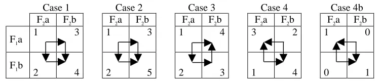
and the concept of evolution as a combinatoric optimisation process on a rugged landscape [14], provides the now familiar model at the heart of the issues addressing evolvability. Ruggedness in a fitness landscape is introduced by the frustration of adaptive features, or epistasis when referring to the interdependency of genes – that is, it occurs when the ‘selective value’ of one feature is dependent on the configuration of other features. Fitness saddles are created between local optima. The simplest illustration is provided by a model of two features, F₁ and F₂, each with two possible discrete values, a and b, creating four possible configurations: F₁a/F₂a, F₁a/F₂b, F₁b/F₂a, F₁b/F₂b. Table 1, below, gives four exemplary cases for selective values, or fitnesses, for these four combinations. The overlayed arrows in each case show possible paths of adaptation that improve in fitness by changing one feature at a time.

Case 1 Case 2 Case 3 Case 4 Case 4b

F₂a F₂b F₂a F₂b F₂a F₂b F₂a F₂b F₂a F₂b

F₁a 1 3 1 3 1 4 3 2 1 0

F₁b

2 4 2 5 2 3 1 4 0 1

Table 1. Example selective values for combinations of two features.

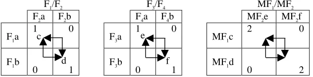
Having established an appropriate two-feature epistasis model, we need an appropriate way to extend it to describe epistasis between a larger number of features. In particular, we want to re-use the same structure at a higher level so as to create the same kind of epistasis between sets of features as we have here between single features; in this way, we can create a principled method for producing fitness saddles of larger scales. Our approach is to describe the interaction of four features F₁, F₂, F₃, F₄, using the interaction of F1 with F2 in one pair, as above, the interaction of F3 and F4 as a second pair similarly,

and then, at a higher level of abstraction, describe the interaction of these two pairs in the same fashion. To do this abstraction we treat the two possible end states of the F₁/F₂ subsystem, i.e. its two local optima (labelled c and d, in Table 2), as two discrete states of an ‘emergent variable’, or ‘meta-feature’, MF1. Similarly, the two possible end states of

the F₃/F₄ subsystem (e and f) form two states for MF₂. If the original, ‘atomic’ features are interpreted as low-level features of an entity, then a meta-feature may be interpreted as a higher-level phenotypic feature of an entity, or some higher-level property of an entity that determines its interaction with other entities and/or its environment.

In this manner we may describe the interaction of the two subsystems as the additional fitness contributions resulting from the epistasis of MF₁ and MF₂. Since each meta-feature includes two ‘atomic’ features, we double the fitness contributions in the inter-group interaction. Table 2 illustrates.

F₁/F₂ F₃/F₄ MF₁/MF₂

F₂a F₂b F₄a F₄b MF₂e MF₂f

F₁a 1 0 F₃a 1 0 MF₁c 2 0

F1b

0 1 F3b 0 1 MF1d 0 2

Table 2. Abstracting the interaction of two pairs of features, F1/ F2 and F3/F4, into the interaction of two ‘meta-features’ MF1/MF2.

The fitness landscape resulting from this interaction at the bottom level, together with the interaction of pairs at the abstracted level, produces four local optima altogether. Using a=0 and b=1, we can write these four optima as the strings 0000 and 1111, which are equally preferred, and, 0011 and 1100, which are equally preferred but less so. Naturally, we can take the two best-preferred configurations from the F_1…4 system and describe a similar interaction with an F_5…8 system, and so on. Equation 1 below, describes the fitness of a string of bits (corresponding to binary feature values, as above) using this construction. This function, which we call Hierarchical If-and-Only-If (HIFF), was first introduced in previous work as an alternative to functions such as ‘The Royal Roads’ and ‘N-K landscapes’, (see [15]).

F(B)= î  

 1,

|B| + F(BL) + F(BR), F(BL) + F(BR),

if |B|=1,

if (|B|>1) and (∀i{bi=0} or ∀i{bi=1})

otherwise. Eq.1

where B is a set of features, {b₁,b₂,...b_k}, |B| is the size of the set=k, b_i is the ith element of B, B_L and B_R are the left and right subsets of B (i.e. B_L={b₁,...b_k/2}, B_R={b_k/2+1,...b_k}). The length of the string evaluated must equal 2p where p is an integer (the number of hierarchical levels).

e f c

A 64-feature landscape using HIFF, as used in our experiments, has 232

local optima (for adaptation changing one feature at a time) [16], only two of these give maximal fitness. To jump from either of the second-best optima (at half-ones and half-zeros) to either global optimum requires changing 32 features at once. Thus, an algorithm using only mutation cannot be guaranteed to succeed in less than time exponential in the number of features [16]. A particular section through the fitness landscape is shown in Figure 1 – the section runs from one global optimum to the other at the opposite corner of the hyperspace (see [13]). As is clearly seen in the fractal nature of the curve in Figure 1, the local optima create fitness saddles that are scale-invariant in structure: that is, the nature of the ruggedness is the same at all resolutions.

0 10 20 30 40 50 60

300 350 400 450

(all−zeros) number of leading ones (all−ones)

fitness

Fig. 1. A section through a ‘scale-invariant’ HIFF fitness landscape.

The hierarchical structure of the HIFF landscape makes the problem recursively decomposable. For example, a 64-feature problem is composed of two 32-feature problems, each of which has two optima. If both of these optima can be found for both of these subproblems then a global optima will be found in 2 of their 4 possible combinations. Thus, if this decomposition is known, then the search space that must be covered is at most 232 + 232 + 4. Compared with the original 264 configuration space, even this two-level decomposition is a considerable saving. In addition, each size 32-problem may be recursively decomposed giving a further reduction of the search space. In [16] we describe how an algorithm having some bias to exploit the decomposition structure (using the adjacency of features on the string) can solve HIFF in polynomial time. Here however, we are interested in the case where the decomposition structure is not known. We call this the ‘Shuffled-HIFF’ landscape [15] because this preferential bias is prevented by randomly re-ordering the position of features on the string such that their genetic linkage does not correspond to their epistatic structure (see [17]).

In summary, this landscape exhibits local optima at all scales, which makes it very challenging to adaptation, and fundamental to the issues of saddle-crossing and scalable evolvability. Moreover, it is amenable to a ‘divide and conquer’ approach if the decomposition of the problem can be discovered and sub-solutions of successive hierarchical levels can be manipulated and recombined appropriately.

3 The Composition model

SEAM manipulates strings of binary features, corresponding to feature combinations as discussed in the previous section. These strings, each representing a type of entity, have variable ‘size’ in that the number of specified features on the string is variable: for example, in an 8-feature system, F₃bF₅a is represented by the string “--1-0---”, where “-” represents a “null” feature for which the entity has no value, or is neutral. The primary mechanism of the model is a mechanism of composing two partial strings together to form a new composite entity. This is illustrated in Figure 2. Such a mechanism assumes the availability of a means of symbiotic union such as the formation of a cell membrane, horizontal gene-transfer [19,20], endosymbiosis [4], allopolyploidy (having chomosome sets from different species) [21], or any other means of encapsulating genetic material from previously independent entities such that they will be co-dispersed in future. However, assuming the availability of such a mechanism does not preclude the interesting biological question of when such a mechanism would provide an adaptive advantage, and when such a union will be selected for.

A: ----1---0—1-- A: ----1----00-1--

B: --1--0---0--- B: --1-0---0-1----

A+B: --1-10---00--1-- A+B: --1-1---000-1--

Fig. 2. ‘Symbiotic composition’. Left) Union of two variable size entities, A and B, produces a

composite, A+B, that is twice the size of the donor entities with the sum of their characteristics. The composite is created by taking specified features from either donor where available. Right) Where conflicts in specified features occur we resolve all conflicts in favour of one donor, e.g. A.

Algebraically, we define the composition of two entities A and B, as the superposition of A on B, below. A={A₁,A₂,…A_n}, is the entity where feature F_i takes value A_i. S(A,B) is the superposition of entity A on entity B, and s(a,b) is the superposition of two individual feature values, as follows:

S(A,B)= S({A₁,A₂,…A_n},{B₁,B₂,…,B_n}) = {s(A₁,B₁),s(A₂,B₂),…,s(A_n,B_n)}, Eq.2. where, s(a,b)=a, if a ≠ null, s(a,b)=b, otherwise. Having defined a variation operator that defines a union of two entities we need to determine whether such a union would be selected for. Our basic assumption is that the symbiotic relationship must be in the ‘selfish’ interest of both the component entities involved. That is, if the fitness of either component entity is greater without the proposed partner than it is with the proposed partner then the composite will not be selected for. If, on the other hand, the fitness of both component entities is greater when they co-occur then the relationship is deemed stable and will persist. But, the fitness of any entity is dependent on its environmental context; possibly, in one environment an entity may be fitter when co-occurring with the proposed symbiont, and in another context the symbiont may depreciate their fitness. Thus whether a symbiotic relationship is preferred or not depends on what environmental contexts are available. For our purposes, the set of possible environmental contexts is well defined: an environmental context is simply a complete set of features (Figure 3).

---0-11---110--- x, an entity specifies a partial set of feature values.

0110101100010011 θθ, an ‘environmental context’ is a complete set of features.

0110111100110011 S(x,θθ), the entity x superimposed on the context θθ.

We assume that the overall fitness of the entity will be a sum of its fitness over different environmental contexts weighted by the frequency with which each environment is encountered. But, we would not generally suppose that the frequencies with which different environments are encountered by one type of entity would be the same as the frequencies relevant to a different type of entity. For example, a biased distribution over environmental contexts may be ‘inherited’ by virtue of the collocation of parents and offspring, or affected by the behavioural migration of organisms during their lifetime, or the selective displacement of one species by another in short term population dynamics. We did not wish to introduce such factors and accompanying assumptions into our model. But fortunately, the concept of Pareto dominance is specifically designed for application in cases where the relative importance of a number of factors is unknown [21]. Put simply, this concept states intuitively that, even when the relative weighting of dimensions is not known, the overall superiority of one candidate with respect to another can be confirmed in the case that it is non-worse in all dimensions and better in at least one. More exactly, ‘x Pareto dominates y’ is written ‘x >> y’, and:

x >> y ⇔ {∀θθ : csf(x,θθ) ≥ csf(y,θθ)} ∧{∃θθ : csf(x,θθ) > csf(y,θθ)}

where, for our ecological application, csf(p,q) is the ‘context sensitive fitness’ of entity

p in context q. So crudely, if x is fitter (or at least as fit as) y in all possible environments

then, regardless of the weightings of the environments for each entity we know that the overall fitness of x is greater than that of y. This pair-wise comparison of two entities over a number of contexts will be used to determine whether a symbiotic union produces a stable composite. If we write the union of entities a and b as a+b, then using the notion of Pareto dominance, a+b is stable if and only if a+b >> a, and a+b >> b. In other words,

a+b is unstable if there is any context in which either a or b is fitter than a+b.

i.e. stable(a+b, a, b) ≡ (a+b >> a) ∧ (a+b >> b),

i.e. unstable(a+b, a, b) ⇔ {∃θθ∈C: (csf(a,θθ) > csf(a+b,θθ)) ∨ (csf(b,θθ))> csf(a+b,θθ))}, where C is a set of complete feature specifications. For our purposes, csf(x,θθ) >

csf(y,θθ) ⇔ f(S(x,θθ)) > f(S(x,θθ)), where f(w) is the objective fitness of the complete

feature set w as given by the fitness function. Thus our condition of instability becomes:

unstable(a+b, a, b) ⇔ {∃θθ∈C: (f(S(a,θθ)) > f(S(a+b,θθ))) ∨ (f(S(b,θθ)) > f(S(a+b,θθ)))}

Eq.3.

We will build each context in the set of contexts by the temporary superposition of other members of the ecosystem. Algebraically, we define a context using the recursive function S*, from a set of n≥2 entities X1, X2,… Xn, as follows:

S*( X₁, X₂,… X_n) =

{

S(X₁, X₂), otherwise. Eq.4.

where S(X₁, X₂) is the superposition of two entities as per Eq.1 above. Some contexts may require more or less entities to provide a fully-specified feature set. In principle, we may use all entities of the ecosystem, in random order, to build a context - but, after the context is fully-specified, additional entities will have no effect. This allows us to write a context as S*(E), where E is all members of the ecosystem in random order. Implementationally, we may simply add entities until a fully-specified set is obtained.

that rapid non-heritable variation (lifetime learning or the temporary groups formed for contexts) guides a mechanism of relatively slow heritable variation (genetic mutation or composition). In other words, evaluation of entities in contextual groups ‘primes’ them for subsequent joins, or equivalently, solutions found first by groups are later canalised [9] by permanent composite entities.

Figure 4 uses Equations 2, 3 and 4 to define a simple version of the Symbiogenic Evolutionary Adaptation Model.

• Initialise ecosystem, E, with random, single-feature, entities. • Repeat until stopping condition:

- Remove two entities at random from the ecosystem →→ a & b. - Produce their union, a+b=S(a,b), using composition (see Eq.2).

- If unstable(a+b, a, b) return a and b to ecosystem, else add a+b to ecosystem. where (as in Eq. 3)

unstable(a+b, a, b) ⇔ {∃θθ∈C: (f(S(a,θθ)) > f(S(a+b,θθ))) ∨ (f(S(b,θθ)) > f(S(a+b,θθ)))} and C is a random set of contexts each built using S*(E) (see Eq.4).

Fig. 4. Pseudocode for a simple version of SEAM.

In the implementations used in the following experiments the maximum number of contexts used in the stability test is 50 (although unstable joins are usually detected in about 6 trials on average). Since the Pareto test of stability abstracts away all population dynamics, only one instance of each type of entity need be maintained in the ecosystem. Initialisation needs to completely cover the set of single-feature ‘atoms’ so that all values for all features are available in the ecosystem. This can be done systematically, or as in our experiments, by over-generating randomly and then removing duplicates.

4 Experimental Results

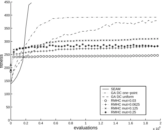
problem size of 64 bits gives a maximum fitness of 448. The data for SEAM are terminated when all runs have found both global optima.

As Figure 5 shows, the results for SEAM are clearly qualitatively different from the other algorithms: Whereas innovation by mutation and by conventional evolutionary algorithms becomes increasingly more difficult as evolution continues in this problem, innovation by composition progresses unimpeded through successive hierarchical levels, and actually shows an inverted performance curve compared to the other methods.

0 0.2 0.4 0.6 0.8 1 1.2 1.4 1.6 1.8 2

x 106 0

50 100 150 200 250 300 350 400 450

evaluations

fitness

SEAM GA DC one−point GA DC uniform RMHC mut=0.03 RMHC mut=0.0625 RMHC mut=0.125 RMHC mut=0.25

Fig. 5. Performance of SEAM, regular GA with Deterministic Crowding (using one-point and

uniform crossover), and Random Mutation Hill-Climbing, on Shuffled HIFF. Error bars are omitted for clarity, but the differences in means are, as they appear, significant.

5 Discussion and Conclusions

contextual evaluation) that scales-up with the size of extant entities; and divide and conquer problem decomposition by combining together solutions to small sets of features to find solutions to larger sets of features.

Some or all of these characteristics could conceivably be provided by other mechanisms. Investigation of these concepts provides valuable insight for issues of evolvability and our model shows that there is a way in which these interesting characteristics could be provided by composition. We suggest that this algorithmic perspective on the formation of higher-level entities, from the composition of simpler entities, provides a useful facet in our understanding of the evolutionary impact of the Major Evolutionary Transitions.

References

1. Buss, LW,1987, The Evolution of Individuality, Princeton University Press, New Jersey. 2. Maynard Smith, JM & Szathmary, E, 1995 The Major Transition in Evolution, WH Freeman. 3. Michod, RE 1999. Darwinian Dynamics, Evolutionary Transitions in Fitness and

Individuality. Princeton Univ. Press.

4. Margulis, L, 1993 Symbiosis in cell evolution, 2nd ed, WH Freeman and Co. 5. Wright, S. 1931, Evolution in Mendelian populations. Genetics 16: 97-159.

6. Wright, S, 1977, Evolution and the Genetics of Populations, Volume 3, U. of Chicago Press. 7. Gould, SJ & VRBA, E, 1982, “Exaptation - a missing term in the science of form”,

Paleobiology, 8: 4-15. Ithaca

8. Kimura, M. 1983, The Neutral Theory of Molecular Evolution, Cambridge University Press. 9. Conrad, M, 1990, "The Geometry of Evolution." BioSystems 24 (1990): 61-81.

10. Waddington, CH, 1942, "Canalization of development and the inheritance of acquired characters", Nature 150: 563-565.

11. Lewontin, RC, 2000 The Triple Helix: Gene, organism and Environment, Harvard U. Press. 12. Cormen, TH, Leiserson, CE, Rivest, RL, 1991 Introduction to Algorithms, MIT Press. 13. Watson, RA, & Pollack, JB, 1999, “Hierarchically-Consistent Test Problems for Genetic

Algorithms”, procs. of 1999 CEC, Angeline, et al. eds. IEEE Press, pp.1406-1413. 14. Wright, S, 1967, “Surfaces of selective value”, Proc. Nat. Acad. Sci. 58, pp165-179 (1967). 15. Watson, RA, Hornby, GS & Pollack, JB, 1998, “Modeling Building-Block Interdependency”,

procs. of PPSN V, Springer 1998, pp.97-106 .

16. Watson RA, 2001, "Analysis of Recombinative Algorithms on a Non-Separable Building-Block Problem", Foundations of Genetic Algorithms VI, 2000, Martin WN, & Spears WM, Morgan Kaufmann.

17. Watson, RA, & Pollack, JB, 2000, “Symbiotic Combination as an Alternative to Sexual Recombination in Genetic Algorithms”, procs. PPSN VI, Schoenauer et al. Springer, 425-434. 18. Fonseca, CM, Fleming PJ, 1995, “An Overview of Evolutionary Algorithms in Multiobjective

Optimization”, Evolutionary Computation, Vol. 3, No.1, pp.1-16.

19. Mazodier, P, and Davies, J, 1991, “Gene transfer between distantly related bacteria”, Annual Review of Genetics 25:147-171.

20. Smith, MW, Feng, DF, & Doolittle, RF, 1992, “Evolution by acquisition: the case for horizontal gene transfers”, Trends in Biochemical Sciences 17(12):489-493.

21. Werth, C.R., Guttman, S.I. & Eshbaugh, W.H. (1985) “Recurring origins of allopolyploid species in Asplenium” Science 228, 731-733.

22. Baldwin, JM, 1896, “A New Factor in Evolution,” American Naturalist, 30, 441-451.

23. Watson, RA, & Pollack, JB, 1999, “How Symbiosis Can Guide Evolution”, procs. of ECAL V, Floreano, D, Nicoud, J-D, Mondada, F, eds. Springer, 1999.

24. Watson, RA, Reil, T, & Pollack JB 2000, “Mutualism, Parasitism, and Evolutionary Adaptation”, procs. of Artificial Life VII, Bedau, M, et al. eds.