Towards a generic model for audit trails

MASTER THESIS

Towards a generic model for audit trails

T. Harleman

Department of Computer Science

August, 2011

Examination Committee

dr. I. Kurtev, University of Twente dr. L. Ferreira Pires, University of Twente ir. R. Zagers, Topicus Finance

3

Acknowledgements

This thesis marks the end of the master ‗Computer Science – Software Engineering‘ of the University of Twente, which I followed since September 2008. This research is performed at Topicus Finance in Deventer where I have worked for about 8 months.

I would like to thank Topicus Finance for the opportunity to do this inspiring and challenging project. A special thanks to my supervisors from Topicus: Robin Zagers, for the technical assistance, feedback and for providing useful suggestions during my research. Further, for the fun at the office, which made the time fly. Jeroen Logtenberg, for endlessly reviewing my work and providing useful suggestions and positive criticism, which kept me sharp.

Also, I would like to thank my supervisors from the university of Twente: Ivan Kurtev, for guiding me throughout the project and providing me with useful suggestions to keep me in the right direction. Luis Ferreira Pires for reviewing my work in great detail, despite the late involvement in the project.

Last but not least, I want to thank my parents for their support during my study and Mark Oude Veldhuis and Martijn Adolfsen, my fellow students, for the good times we had while completing most of the courses.

-Tim Harleman

5

Table of contents

TABLE OF CONTENTS ... 5

1 INTRODUCTION ... 7

1.1 CONTEXT ... 7

1.2 PROBLEM STATEMENT ... 8

1.3 RESEARCH QUESTIONS ... 8

1.4 APPROACH AND OUTLINE ... 9

2 BASIC CONCEPTS ... 10

2.1 AUDIT TRAIL ... 10

2.2 PROVENANCE ... 10

2.2.1 Workflow provenance ... 10

2.2.2 Data provenance ... 11

2.2.3 Provenance and archiving ... 12

2.3 MODELLING PURPOSES ... 13

2.4 MODELING AND LOGGING ... 14

2.5 APPROACHES FOR AUDIT TRAIL ANALYSIS ... 15

2.5.1 Fraud in administrative ERP systems ... 15

2.5.2 Rule-based system for universal audit trail analysis ... 16

2.6 DOMAIN OF MORTGAGES ... 16

2.6.1 Organization ... 17

2.6.2 Process ... 17

3 DATA WAREHOUSE ARCHITECTURES ... 20

3.1 APPROACH ... 20

3.2 NORMALIZED DATABASE ... 21

3.3 OLAP ... 22

3.4 FLUIDDB ... 23

3.5 INFOBRIGHT ... 25

3.5.1 Layers ... 26

3.5.2 Data Manipulation Language ... 26

3.5.3 Example of query handling... 27

3.6 ARCHITECTURE COMPARISON ... 29

3.7 CONCLUSION ... 31

4 DATA WAREHOUSE DESIGN ... 32

4.1 APPROACH ... 32

4.2 AUDIT TRAIL LOG ANALYSIS ... 32

4.3 DATA WAREHOUSE CONVERSION ... 33

4.3.1 Conversion rules and exceptions ... 34

4.3.2 Data warehouse schema ... 35

4.4 TEST CONVERSION RESULTS ... 36

4.5 DISCUSSION ... 38

4.6 CONCLUSION ... 38

5 AUDIT TRAIL QUESTION MODEL ... 40

5.1 APPROACH ... 40

5.2 GENERIC MODEL ... 40

5.3 POSSIBLE AUDIT TRAIL QUESTIONS... 41

6

5.5 LABELING ... 42

5.6 QUESTION META MODEL ... 43

5.7 CONCLUSION ... 44

6 AUDIT TRAIL ARCHITECTURE... 45

6.1 ARCHITECTURE ... 45

6.2 QUESTION PARSER ... 46

6.3 LABELBASE ... 48

6.4 LABEL RESOLVER ... 50

6.5 DATABASE LAYER ... 52

6.6 POST PROCESSING LAYER ... 54

6.7 POSSIBILITIES AND LIMITATIONS BEYOND REQUIREMENTS ... 54

6.8 CONCLUSION ... 55

7 PROTOTYPE ... 56

7.1 APPROACH ... 56

7.2 REQUIREMENTS ... 56

7.3 DESIGN ... 57

7.4 IMPLEMENTATION ... 58

7.4.1 User Interface ... 58

7.4.2 Query generation ... 59

7.5 PERFORMANCE TEST ... 60

7.5.1 Test Approach ... 61

7.5.2 Test suite ... 62

7.5.3 Test results ... 63

7.6 DISCUSSION ... 64

7.7 CONCLUSION ... 67

8 CONCLUSION AND FUTURE WORK ... 69

8.1 SUBQUESTIONS ... 69

8.2 MAIN QUESTION ... 70

8.3 FUTURE WORK ... 71

REFERENCES ... 72

APPENDIX A ... 73

APPENDIX B ... 74

APPENDIX C ... 75

7

1

Introduction

Financial applications that support processes involving money, like banking applications, need to be fault proof. To gain the trust of customers, financial companies spend a lot of time, money and resources on validating their software. Systems that concern money or health require a higher degree of fault proof systems then systems that don‘t.

Within the domain of mortgages, banks and mortgage companies loan money to clients so that they can finance a house. When a person wants to buy a house, generally they have to go to a mortgage company to get a mortgage for the house. Getting a mortgage involves a lot of paperwork and requires a variety of information about the current and historical financial situation of the buyer. For example, the buyer has to supply information about his yearly income, if the buyer has or had other loans, identification documents and so on. The mortgage company on their turn has a lot of different mortgage products. There are life insurance mortgages, linear mortgages, mortgages with a variable interest or mortgages where money is invested. These days there are over a hundred different mortgage products, often in combination with insurances. In order to keep track of all provided mortgages, with all these complex products and insurances, software systems are necessary.

Software that is used in this process has to be reliable for both parties involved. From the client‘s point of view, all information about their mortgage should be correct, such as interest, satisfied payments, interest rate, mortgage products, insurances and so on as been agreed upon during the negotiations. From the view of the mortgage company, the system should keep correct records about all the provided mortgages. When such system contains faults, the company could lose money because of incorrect interest rates or by paying out insurances that a client does not have. On the other side, the company has to be able to ensure the data is correct and be able to verify this to its clients. This could be the case when a client claims he paid his monthly payment or that a mortgage product is different than what was agreed upon during the negotiations.

Proving the correct information is stored is an important factor in financial systems. A common approach within administrative applications is the use of audit trails. Audit trail is a logging strategy which makes it possible to store and retrieve information about changes made in the process of creating the mortgage invoice. An audit trail can provide a complete history of how the end product is formed by backtracking the historical data of changes. However, strategy focuses more on storing and less on retrieving the historical information.

1.1

Context

8

logs can be used for functionality like fraud detection. Currently, when Topicus wants to query the audit trail, the database server crashes or the query gets a time out. Either way, no results are obtained from the audit trail. Because of poor performance, this research has focused on how we can improve the current use of the audit trails within Topicus and how to make the data questionable with acceptable performance, in units of time.

1.2

Problem statement

Some clients and Topicus Finance themselves are SAS 70 [1] certified. This standard prescribes that the client and Topicus Finance must define a that justifies the data in their current database. For this they use an Audit Trail. The audit trail logs every database change, made in the application in a separate database. With this log, the clients and Topicus can justify the current state of for example, a field within the database, by retrieving historical information. Further, with this log they can reconstruct the database state at any point in time.

The problem is that the audit trail was optimized to store. Later, clients asked for

functionality to be able to retrieve information from the audit logs. Due to this change in requirements, the audit trail implementation now has poor structure and performance to meet the requests of the clients. The audit trail logs a lot of data

without being able to retrieve any information from the logs within reasonable time. To get information from the audit trail, the data has to be distributed into multiple smaller databases in order to get any results at all. The data set is too large for the database server to handle in its current database schema. Therefore, functionality for the audit trail data cannot be added to their applications as requested by their clients.

1.3

Research Questions

In this section we propose the research questions which we have addressed during this research. This research has aimed at finding a solution, in the form of a design, which makes it possible to question the audit trail data with a better performance than the current audit trail.

What is a generic architecture for efficient questioning of audit trail logs?

1. What is an audit trail?

We have introduced the concept of audit trails in Section 1.1. More information about audit trails can be found in [2].

2. What data warehouse architecture is suited for storing audit trail logs?

3. What is a generic architecture for handling audit trails?

a. What meta data is required by the architecture in order to

understand the data?

b. How should a (generic) model, to represent audit trail data, look

9

c. What architectural changes to the architecture or model have to

be made in order to make it domain specific for any domain?

To efficiently go through a large bulk of data, extra information, called meta data, is commonly used to group and find data faster and more efficiently. In previous research [2], we have seen that data provenance uses the notion of labeling to label data in order to address data by referring to its labels.

4. What is the performance increase (measured in units of time) of the

proposed architecture?

In order to verify the performance of the proposed solution for the business case, we have implemented the architecture in a prototype. By running tests, the architecture could be compared with the performance of the current audit trail implementation.

1.4

Approach and Outline

In order to answer the research questions mentioned in Section 1.3, we start with some preliminaries in Chapter 2, which give an introduction to the terms Audit trail, provenance, data warehousing, modeling and modeling concepts.

In order to find a suitable data warehouse architecture and to answer the third research question, we did some research on several types of data warehouse architectures. We compared these architectures based on relevant criteria and chose an architecture. The comparison is described in Chapter 3.

To see if practice matches the theory, a simple test was performed to see how the architecture would perform for this business case. A data conversion is performed to obtain information about the data storage efficiency of the new architecture compared to the current situation. All of that is described in Chapter 4.

To answer the fourth research question, first, a definition for the term „generic

model‟ is given. Interviews were held to find out what types of questions are going to be asked about the audit trail data and what output is expected. From that, we abstract from the domain specific parts to design a model that could, ideally, be applied on any type of logging. While abstract from the domain, we kept in mind that the amount of architectural changes for a domain specific design should be kept at a minimum. Last, a solution regarding meta data is required to let the generic model understand what data it handles. All of that is described in Chapter 5.

Chapter 6 describes the audit trail architecture in more detail. We zoom in on every component in the model to show the responsibilities and how it works internally, specifically for our business case.

To be able to say anything about the performance of the model we implemented a small prototype. By running some example questions we compared the results, in units of time, with the current implementation of the audit trail. From these results and observations made during prototyping, we drew some conclusions about the performance of the model. The prototype and test results can be found in Chapter 7.

10

2

Basic Concepts

This chapter discusses the basic concepts that the reader should be familiar with to fully understand the terms and techniques used in this thesis.

Organization of this chapter Section 2.1 explains the term audit trail, Section 2.2 introduces the term provenance, what it is and how it is used. Section 2.3 talks about why there is need for a model for software in general. Section 2.4 focuses on what modeling can add to logged data. Section 2.5 shows some approaches of how the audit trail is used in practice. Last, Section 2.6 gives an introduction to the domain of mortgages and the process of getting a mortgage.

2.1

Audit Trail

We consider the definition of the concept ‗Audit Trail‘ from [3]:

“An audit trail or audit log is a chronological sequence of audit records, each of which contains evidence directly pertaining to and resulting from the execution of a business process or system function.”

In the context of this research an Audit Trail is a log that holds all changes made to a database, usually changes made by users of a system. A big problem with this form of logging, as with almost all forms of logging, is that the logs grow very big, very quickly. This is often compensated by selective logging or keeping the logs for shorter periods. Our business case consists of a situation where there is no room for compensations and all data needs to be logged for a long period. With this research we aim at finding a solution to obtain information from these large audit logs.

2.2

Provenance

Since logging, like an audit trail, easily grows out of manageable proportions, we need some data storage structure to keep some performance on the long run and that can support the storage and retrieval of historical data. For that, we look into

data provenance. Provenance (also referred to as lineage or pedigree) means origin

or source. Some call it “the history of ownership of a valued object or work of art

or literature”[4]. From a scientific point of view, data sets are useless without knowing the exact provenance and processing pipeline used to produce derived data sets. In relation to our problem, when an invoice for a mortgage is created it is valuable knowing what data is altered during the process of creating the invoice.

We look into two flavors of provenance, namely workflow provenance and data provenance to determine which seems more applicable to our problem.

2.2.1 Workflow provenance

11

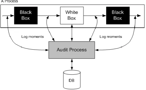
particular dataset. Sometimes records are kept about software versions, brand and models of hardware and use of external software within the workflow. When using external processes within the workflow provenance is usually coarse-grained, which means, that only the input, output and external software is recorded. Those external processes are seen as black boxes.

The idea is shown in Figure 1 below. The audit process logs information on the log moments, indicated with vertical arrows. With black boxes in the process, the only log moments are before and after the black box. White boxes can have internal log moments. Workflow provenance logs more snapshots of the data at the log moments rather than the explicit changes.

Figure 1: Workflow example

2.2.2 Data provenance

Data provenance gives a more detailed insight about the derivation of a piece of data that is the result of some transformation step. In our scenario, the resulting product could be the mortgage invoice. A particular case of data provenance is very popular within the database community and is extensively researched, which is the when this transformation is performed by database queries. The following

explanation comes from [20]. Suppose a transformation on a database D is

specified by query Q, the provenance of a piece of data i in the output of applying

Q on D is the answer to the following question: ―Which parts of the source

database D contribute to i according to Q?‖ We can further categorize this into

where- and why- (or how-) provenance.

 Where-provenance identifies the source elements where the data in the

target is copied from.

 Why-provenance describes why a piece of data is present in the output.

Sometimes why-provenance is referred to as ‗how‘-provenance and some authorsdefined it as a variant of why-provenance. We ignore this variant in this research.

We explain these categories by means of an example derived from [5].

Suppose ("Jan", 657) is an answer to the following query on the tables shown below.

Select name, telephone

From employee e, department d

12

Employee Department

id name id emp_id name phonenumber

1 Jan 11 1 Computer Science 657

2 Henk 12 2 Embedded Systems 739

The where-provenance of the name ‗Jan‘ is simply the corresponding record in the name tuple of the Employee table. It only tells you where the data is copied from. This is marked in the table above. The why-provenance includes not only the record in the employee table, but also the Computer Science record corresponding to its employee id. Without the department record, ‗Jan‘ would not be included in the result set. These records are marked in the table above.

Data provenance has two general approaches, namely annotated and non-annotated. Non-annotated provenance calculates the provenance using the input, output and query where the annotated provenance can be calculated lateron using extra information that is stored after the execution of a query. The problem with annotated provenance is that it adds a lot of overhead and might be less suitable for very large data sets. The positive side is that it gives more control about what data is more important by annotating it. The downside of non-annotated provenance is that calculations can only be performed during query execution. Afterwards new information cannot be added, unlike the annotated approach where annotations can be added at any time.

2.2.3 Provenance and archiving

Within data provenance, there is a notion of archiving. With the audit log, structural changes of the database can be expected and therefore should also be considered in the solution.

13

Figure 2: Archiving structural database changes

In our scenario we consider two databases: The production database where applications run on and which holds the most recent information (Table C in Figure 2), and the Audit trail database which is responsible for holding the logged information. Table A contains the logged information about Table C. Every record has an additional column with a timestamp indicating when a change occurred. Table B holds the structural changes about Table A, in which we can see which

columns were added, deleted or changed. We have a function f(x), which takes a

timestamp as value for ‟x‟ to calculate the state of a record or table during the given

point in time x.

Assuming we would like to retrieve the values of the record of the application

with „app_id = 101‟ at f(20-12-2010 11:45). From Table B we conclude that

column „attr_3‟ was not included at that point in time, but „attr_2‟ would be

present. From Table A we see that the deletion of „attr_2‟ did not occur yet before

11:45. The result is therefore, (101, 1002, 5.05).

Assuming we would ask the same question again, but now for „x = 20-12-2010

12:10‟. From table B we conclude that „attr_3‟ was added and thus should the value for this column be included in the result. From Table A we see that some changes have been made before 12:10. The result is therefore (101, 1002, 5.09, 401).

From the archiving point of view this approach works. A detailed registration is held about the structural changes of the application and is easily retrievable. Nevertheless, the storage of Table A is inefficient since it holds a lot of redundant information. This example explains how the archiving of structural database changes can be recorded. How the content is stored is a different point of concern.

2.3

Modelling purposes

14

Modeling is often used in the process of designing software. Small projects do not necessarily need a model before building the real system. These types of small projects mostly share the following five characteristics [6];

1. The problem domain is well known.

2. The solution is relatively easy to construct.

3. Very few people need to collaborate when building or using the system.

4. The solution requires minimal ongoing maintenance.

5. The scope of future needs is unlikely to grow substantially.

Larger projects, that do not have the characteristics above, usually require a some sort of model. There is always a possible tradeoff to model a system or build it straight away. The tradeoff is based on the complexity of the project and, the risk of building software without making a modeling. Modeling provides architects and others with the ability to visualize entire systems, assess different options and communicate designs more clearly before taking on the risks —technical, financial or otherwise — of actual construction. Some software systems support important health-related or money-related functions, making them complex to develop, test and maintain. These days, software become more and more important for almost any business process. Therefore, developers need a better understanding of what they are building. Modeling is an effective way increase the understanding. More specifically, by modeling software, developers can:

 Create and communicate about software designs before committing

additional resources.

 Trace the design back to the requirements, helping to ensure that they

are building the right system.

 Practice iterative development, in which models facilitate quick and

frequent changes.

2.4

Modeling and logging

To be able to retrieve information from large datasets like audit trail logs, the structure of the data is an important aspect. Structuring large datasets has a few advantages. Structured logs, or databases in our case, are readable to some extent. Structure provides better understanding of the content, which facilitates the design of software or models to give purpose to the data. In practice, several purposes for audit trails can be found. For example, the logs can be used as logs as intended, thus when something goes wrong and the cause needs to be found. Another purpose which seems to become more popular is analysis of audit trails and other logs. In this report we define two types of analysis:

Passive analysis: A combination of questioning the logs for e.g. tracing problems and using the logs to generate statistics or use it for data mining.

Reactive analysis: Done real-time and can be used to detect errors made by the user and generate a notification..

15

2.5

Approaches for audit trail analysis

A lot of approaches, concerning audit trails, focus on the areas of intrusion detection and fraud detection. Audit trail are generally monitored and analyzed to build up a dataset. This dataset is used to compare real-time actions in a particular software system to detect fraud or intrusion by comparing the actions with what is known or expected behavior. In the following sections, some approaches are discussed.

2.5.1 Fraud in administrative ERP systems

In financial and administrative applications, logging analysis is used mainly to detect or prevent any form of fraud. In [7], P. Best refers to five essential steps for detecting fraud in software systems.

1. Understanding the business or operations.

2. Performing a risk analysis to identify the types of frauds that can occur.

3. Deducing the symptoms that the most likely frauds would generate.

4. Using computer software to search for these symptoms.

5. Investigating suspect transactions.

In [7] they use audit trails as a means to detect fraud in ERP (Enterprise Resources Planning) systems. ERP systems are software systems in which administrative information is stored about the company. ERP systems can be centralized so that there is one administrative system for large companies with multiple settlements in different cities or countries.

P. Best,[7], focuses on fraud in such administrative systems. To do so, they define various types of audit trails. Security audit trails log information of user activity to the system. These logs often include successful logins, failed logins, starting of a transaction or action, failed starts of (trans)actions (i.e. prevented because of role permissions) and changes in roles. Usually these audit trails may be retained for periodic review, then archived and/or deleted. Accounting audit trails log specific information concerning financial transactions, like who does payments, when are they performed, who made the payments, who checked financial balances and so on. With this log the financial companies can backtrack every payment that is performed or viewed within the system. [7] defines an audit trail approach to support detection of fraud. The approach consists of two stages:

1) threat monitoring, which involves high-level surveillance of security audit logs to detect possible ‗red flags‘. To decide what a possible threat is, they use the audit logs to build up a profile of each user over a certain time period. This profile gives an indication of the frequently performed actions of a user, or patterns in the actions. A knowledge base system may also be developed to generate forecasts of expected user activity. Changes in actual user behavior may then be detected promptly and investigated. The forecast of predicted actions can be improved by creating user profiles in a smaller time frame and compare this to see shifts in the profile. For example, a user can perform different actions in the beginning of the week than at the end of the week.

16

2.5.2 Rule-based system for universal audit trail analysis

The University of Namur in cooperation with Siemens Nixdorf Software S.A. developed a rule based language for universal audit trail analysis for UNIX. The language is called RUSSEL [8] (Rule-baSed Sequence Evaluation Language) and tailored to the problem of searching for arbitrary patterns of records in sequential files, like audit trails. The built-in mechanism allows records to pass the analysis of the sequential file from left to right. The language provides common control structures, such as conditional, repetitive and compound actions. Primitive actions include assignments, external routine calls and rule triggering. A RUSSEL program consists of a set of rule declarations that are identified by a rule name, a list of formal parameters and local variables and an action part. The action part can consist of user-defined or built-in C-routines. A simple and clearly specified interface with C allows users to extend the RUSSEL language with any desirable feature. This can include simulation of complex data structures, specifications of alarm messages (mail, text message, popup), locking a user account and so on.

When analyzing audit trail logs, the system executes all the active rules on every record. The execution of an active rule may trigger or activate new rules, raise alarms, write report messages or alter (global) variables. Rules can be activated for the current record or the next. Once all rules are executed for a single record, a new record is obtained from the log and all rules return to their initial state. This means that, rules that were triggered to be active become inactive again unless triggered to stay active. The abstract syntax of RUSSEL can be found in [8]. Example rules can be found in [9]. The operational semantics of the RUSSEL language can be summarized as follows:

 Records are analyzed sequentially. The analysis of records consists of

executing all active rules. An active rule can trigger other rules, raise alarms, write report messages, alter variables etc.

 Rule triggering is a special mechanism by which a rule is made active

either for the current or the next record. In general, a rule is active for the current record because a prefix of a particular sequence of audit records has been detected. The rest of the sequence has to be possibly found in the rest of the log. Parameters in the set of active rules represent knowledge which is obtained from the already analyzed records. This knowledge is used while analyzing the rest of the records.

 When all the rules active for the current record have been executed, the

next record is read and the rules triggered for this record in the previous step are executed in turn.

 To initialize the process, a set of so-called initialization rules are made

active for the first record.

2.6

Domain of mortgages

17

2.6.1 Organization

In order for a mortgage company sell mortgages to clients, there are a few parties involved. The mortgage company also needs ways to be profitable and gain its money. Figure 3 indicates of the involved parties.

Figure 3: Global organization of a mortgage company (from [10])

Within mortgage companies, three offices are usually defined, namely Front-,

mid- and back-office. The front-office usually refers to the different sales and distribution channels a mortgage company knows. Some mortgage companies have their own sales department, but outsourcing that activity to different distribution

partners seem to happen more often. Distribution partners are intermediaries or

franchisers. This kind of people sell mortgages for different companies. The

advantage is that consumers (people looking for a mortgage) have more choice in

mortgages from various companies with an ‗independent‘ advice when they visit an intermediary of franchiser. Naturally, mortgage companies give bonuses when an intermediary sells their products. Such bonuses make advice less ‗independent‘. The mid-office performs the process of making offers for consumers, validating the applications and accepting applications. The back-office comes after the mid-office and performs the process after the mortgage deal is closed. It focuses on consumers

paying off their mortgages. Chain partners are specialized companies that can take

over some of the processes of a mortgage company. Examples are outsourcing of the back-office, but also authorities that supervise the mortgage market, like AFM [11]. Like car manufacturers need resources to build cars, mortgage companies also need resources to be able to sell mortgages. Those resources are called financial

means and are gained from the financial market. Traditionally, banks use its clients

savings as resources but mortgage companies are not always banks, thus they need other ways for getting money.

Nowadays, mortgage companies sell their mortgage wallets (a set of mortgages) to third parties. In that way, mortgage companies can directly use money again and the paying off risks now lay at the third party holding the wallet. Another popular approach is ‗securitization‘. Mortgage companies sell their wallet to a so called an SPV (Special Purpose Vehicle), which is a Ltd. Company to be founded. The SPV generally transforms the mortgage wallet into obligations on the stock exchange and sells them. Each SPV is responsible for getting money from its consumers, paying interest and repaying the obligations. When a wallet ends with loss, the obligations with the lowest rating end up with the loss. The higher the ranking of the obligation, the less risk is in case the wallet ends with loss.

2.6.2 Process

18

their products. In Figure 4 a schematic overview of the primary process of a mortgage company is shown. These days, a lot of insurances are sold together with a mortgage. Insurances are not included in the primary process. The primary process describes only the phases that are usually adopted in the processes of the mortgage companies. Variations of this process and perhaps totally different processes. For simplicity, we use this general process to characterize the mortgage process.

Figure 4: Primary process for mortgages

Each phase is discussed below.

Sales – Front office

Advice: The sales of mortgages is done by either a sales department of the bank or mortgage company or by intermediaries and franchisers. Sometimes you see mortgages are sold via the internet. In this phase, the seller tries to find out the needs of the client and an estimation is made whether the client would be accepted by the mortgage company. Based on the needs, a mortgage product is selected and proposed to the client.

Offer – Mid office

Validation: When the client has interest in the mortgage that was proposed during the sales phase, the client can ask for an offer. The mortgage company will validate the application and will check according to a checklist to see if the company can offer the mortgage the client requests. Mostly some background information is looked up about the client and some global financial information from BKR [12]. If the application passes these checks, the offer can be created. A full acceptance check is done later.

Offer creation: In this phase the offer is created and presented to the client.

Acceptance – Mid office

Client Acceptance: The client accepts the conditions described in the offer, signs the documents and sends them back to the mortgage company. Here he formally agrees on his side of the agreement.

19

Bankacceptance: When all the required documents are gathered, the documents are read and checked where necessary. When all documents are checked and accepted, the mortgage company agrees on their side of the agreement for the mortgage offer. The mortgage application is now complete and the client gets access to the money.

Transfer

This phase is about the transfer of the house from seller to buyer.

Mortgage document: The mortgage company sets up a notary instructions document in which the mortgage company describes how the house will be financed. The payment can be fully covered by the mortgage or that a part will be paid by the client. For example, from money that was left over from the sales of another house. This document is also an agreement between the client and mortgage company.

Property transfer: The seller and buyer sign the house-transfer document. The buyer is now officially the new owner of the house.

Register property: Every property has to be registered at the ‗Land register‘ This is a central register in which the property rights and mortgage rights on property are registered.

Management – Back office

Mortgage management: Once the property is officially transferred, the loan of the mortgage is activated. Mortgage management concerns about every action related to paying off the mortgage. An action can be a monthly fee over interest, a payment in between or any amount or changes to the mortgage conditions during the pay off period. This is the standard process.

Debt management: If a client does not pay his mortgage, the client ends up in the debt management. These clients are handled separately from the rest and are monitored more intensively. Once the client catches up with his payment he is transferred back to the standard mortgage management. If the client keeps paying late or not at all, the mortgage company might be forced to sell the property. The profit of sales is for the mortgage company.

Closing

20

3

Data warehouse architectures

A data warehouse is required to store the audit trail data. Therefore we spent some time selecting a suitable data warehouse architecture. This chapter focuses on the selection of a data warehouse architecture that is suitable for working with audit trails in general and how the selected architecture would be applied on our business case.

Organization of this chapter: Section 3.1 describes the approach that aims at answering the second research question. Section 3.2 looks into several data warehouse architectures from which we have made our choice. We discuss the characteristics of each individual architecture. Section 3.3 covers the comparison of the architectures by looking at their strengths and weaknesses and grading them according to the predefined criteria. Last, in Section 3.4 holds the conclusion about the chosen architecture and the results of the comparison.

3.1

Approach

In order to answer the second research question (“What data warehouse

architecture is suited for storing audit trail logs”), the following has been done. We selected four data warehouse architectures. From those four, two are specific products, that have been selected since they implement an interesting variant of a standard architecture, or the underlying architecture is specifically designed for its product. Therefore some product were selected, but the focus is on their underlying architecture. The different architectures are selected based on the differences in the underlying architecture and their theoretical performance. The information about performance is obtained from experts and the (product) developers. Four different

data warehouse architectures and products were selected, namely OLAP,

Normalized Data warehouse, FluidDB [13] (uses EAV data triples [2]) and

InfoBright [14] (which uses compression and a special form of indexing). We will introduce each architecture or product and list their strengths and weaknesses.

The selected data warehouse architectures are compared on several criteria that are relevant for our business case. The architectures are compared according to the following criteria:

 (Analytic) query performance. Most architectures are designed for either analytic or regular queries. We look at how the architectures perform on both these types of queries in relation to each other, as stated by experts and developers. Grading: 1(bad) – 5(very good)

 Maximum data size. Roughly for which the architectures still performs acceptable. Beyond the indicated size, the performance goes down exponentially. Grading: 1(small size) – 5(large size), relative comparison between the architectures and kept in mind an expected audit trail size in the order of 30 to 50 Gb.

 Meta information. Information that is added by the architecture itself. Meta information becomes overhead, unless it is helpful information to our solution. Therefore, meta information forced by the architecture should be limited. Grading: 1(a lot) – 5(none)

 Support to textual data. To what degree the architectures are designed to

handle textual dataGrading: 1(bad) – 5(very good)

21

Audit logs tend to have a very high degree of redundancy, therefore the grading is doubled for this criteria. Grading: 1(A lot) – 10(None)

 Scalability. How the architecture scales, horizontally (addition of servers) and/or vertically (addition of CPU/memory to a server) Grading: 1(bad) – 5(very good)

 Maintainability. How much effort, in units of time, is required to maintain the data warehouse. Grading: 1(bad) – 5(very good)

 Side-effects. Caused by possible insert/update/delete actions. Audit trails log a lot of information. To keep the data warehouse up-to-date, a continuous stream of insertions are performed for new log records. The insertions should not have negative side effects. Grading: 1(None) – 5(a lot)

By looking at the strengths and weaknesses of the different architectures and by giving grades from 1(bad) to 5, or 10(very good) to the criteria above, we got an overall score for each architecture. The scores have been assigned based on literature, known research, opinions of experts or our own knowledge. Based on the score, the appropriate architecture has been selected.

3.2

Normalized database

For the structure of our data warehouse we looked into the field of sensor data storage. Sensors produce a lot of data which needs to be stored and retrieved. Our problem involves less data than sensor storage has to cope with, therefore we think that if a solution works for the storage of sensor data, it would perform well in our case.

The University of Central Florida [15] did a comparison between normalized data warehouses and denormalized data warehouses to show the advantages between the two. Based on their results, when normalizing a database, the number of records increases (records generally have 2 or 3 columns) and the data volume decreases, meaning less size on disk. Since we handle large data sets, we are more concerned in reducing the space on disk rather than the number of records. When normalizing, the costs for administration raises and the labeling takes a little extra storage. Depending on how the data warehouse is set up, this could be an issue. With logs, the redundancy rate is extremely high. By removing redundancy using normalization, the extra costs of the extra administration probably does not add up to the decrease in data size.

Since we do not have to handle the data real-time, the time it takes to populate the warehouse is less of an issue. The last ‗weakness‘ in the comparison from [15] is that transformations on normalized databases are harder. This is true for the general case, since the normalized databases have more tables. Also, a data warehouse should not be used for other purposes than questioning the data in the way the data warehouse was set up. Apart from that, transforming a data warehouse is usually done only once and not on a regular bases. Considerations regarding possible transformations should be known and kept in mind when designing the data warehouse.

22

Comparison

Table 1 shows the evaluation of the normalized data warehouse architecture regarding the criteria, which are defined in Section 3.1

Table 1: Evaluation of the normalized database architecture.

Criteria Evaluation

(score)

Motivation

Query performance Good (4) Normalization is applied to increase the query

performance in general Analytic query

performance

Good (4) Due to the standard functionality (from SQL) to

calculate multi cubes

Scalability Good (4) Tables could be divided over multiple servers and

more memory increase cache size, thus performance

Data redundancy None (10) The goal of normalization is to minimize or

prevent data redundancy

Max. database size 10 – 50 GB (3) Depending on the size of the individual tables,

hardware and difficulty of queries

Meta information None (5) By itself, a normalized database does not generate

meta information about its content.

Textual data Good (4) Textual searches are always slower then numeric

searches, but due to low/no redundancy, the amount of text to be searched is limited.

Side effects None (5) By normalizing a data warehouse, no relevant side

effects appear.

Maintainability Good (4) It has a simple database schema and there is good

tool support for maintenance.

3.3

OLAP

OLAP stands for Online Analytic Processing and is an approach to handle

multi-dimensional analytic queries. OLAP systems generally are used for business intelligence reporting tools and data mining where data cubes are used to retrieve the desired information. OLAP is a sort of layer that runs on top of a normal database. There are three types of OLAP architectures, namely, MOLAP, ROLAP and HOLAP. The biggest weakness is that OLAP products are not suitable for handling data with multi-hierarchical and unbalanced structures. The strength lies in retrieving analytical and statistical information from data sets.

23

does not pre-compute them. ROLAP can be used using normal SQL tools, since it is a layer on top of a normal database, which makes it more generic for average use than having to study OLAP tools in order to work with it. Last, loggings generally contain quite some textual data. ROLAP is said to handle this kind of data pretty well. For all these reasons we select ROLAP as the OLAP representative for our project based on the conducted comparison in[16].

Evaluation

Table 2 shows the evaluation of the ROLAP architecture regarding the criteria defined in Section 3.1.

Table 2: Evaluation of the ROLAP architecture.

Criteria Evaluation

(score)

Motivation

Query performance Good (4) The architecture is designed to obtain information

from large data sets Analytic query

performance

Very Good (5) The multi dimensional cubes improve the

performance of the analytic queries

Scalability Good (4) Tables could be divided over multiple servers and

more memory increase cache size, thus performance

Data redundancy Average (6) When the multi dimensional cubes are stored they

hold copies of the original data.

Max. database size 10 – 50 GB (3) Depending on the size of the individual tables,

hardware and difficulty of queries

Meta information None/Little (4) When multi cubes are calculated and stored, the

cubes hold statistical/analytical information about the content.

Textual data Good (4) Textual searches are always slower than numeric

searches, but due to low/no redundancy, the amount of text to be searched is limited.

Side effects Yes (3) Stored computed multi cubes might have to be

recomputed from time to time.

Maintainability Good (4) It has a simple database schema and proper tool

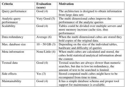
support for maintenance is available.

3.4

FluidDB

24

FluidDB uses an architecture based on Entity-Attribute-Value (EAV) triples, or data triples. The architecture is implemented so that the data is stored in a relational database, and the actual content is stored as compressed XML. Via those triples, the location of the actual content in the compressed XML can be obtained. The EAV architecture is used as a lookup system for the actual content. In FluidDB, there are four key concepts, namely:

 Objects: Represents the actual content

 Tags: Labels attached to objects which define the attributes of objects.

 Namespaces: Organizes or groups tags

 Permissions: Handles access control

Figure 5: FluidDB data format.

The object represents the actual content, the ‗about‘ tag is optional but should be unique and an id can be used to retrieve the actual content. Per object, additional tags can be attached. A tag consists of a namespace followed by the name of the tag, and a value. The data triples consist of an object, a tag and a value. An example of an object is represented in Figure 6:

Figure 6: Visualisation of data triples for an object in FluidDB

25

In our own research [2], we concluded that data triples is not the best architecture for our problem. FluidDB made some improvements to the concept of data triples and showed it can be effective for large sets of data, like tickery. But, the use of cloud computing, makes FluidDB an unsuitable choice. Its architecture is tailored towards social data which is publicly accessible, which is something we do not want looking at the confidentiality of the audit data. Cloud computing is getting more secure for private use, but the client has to have faith in that security. The permission system on the other hand is simple and effective but might get out of hand when permissions need to be set for a lot of users and a huge tag set, especially when the tags can be defined by any user per object. Tag management, therefore, should be managed closely so that it does not get out of hand.

Evaluation

Table 3 shows the evaluation of the FluidDB data triple architecture regarding the criteria defined in Section 3.1.

Table 3: Evaluation of the FluidDB data triple architecture.

Criteria Evaluation

(score)

Motivation

Query performance Good (4) The architecture is designed to obtain small pieces

of information from large datasets. Analytic query

performance

Poor (2) Analyzing the data triples with possible different

labels per object takes a lot of effort.

Scalability Average (3) Good scalability, horizontally due to cloud

computing. Average scalability vertically.

Data redundancy Little (8) Not intended, but the architecture does not restrict

it.

Max. database size 450 – 500 GB

(4)

Data triple architectures are measured in number of triples rather than size. They can handle a few billion triples. A rough indication is 250 kb per triple * 2 billion = 450 – 500 GB

Meta information A lot (1) Tags attached to objects are considered meta

information

Textual data Good (4) Has no limitations that restrict the performance on

textual data lookups

Side effects None (5) The usage of data triples has no unintended side

effects

Maintainability Poor (2) Due to the billion of triples, maintainability

suffers. Tool support is limited.

3.5

InfoBright

Infobright [14] is a company that focuses on analytic data warehouse products. They have a commercial and open source variant of their product called Infobright, named after the company. Infobright gives support especially for very large datasets (up to 50 TB). It combines smart compressions with good performance and low installation and maintenance costs.

26

TeraByte on a single industrial standard database server. About performance and scalability they claim fast load speed, which remains constant as the size of the database grows, fast query speed on large volumes of data and they offer high data compression with a ratios between 10:1 to over 40:1. This results in less storage and less I/O requirements. Another important factor is that Infobright is column oriented and not row oriented as in traditional databases.

3.5.1 Layers

The architecture behind Infobright consists of 3 layers: Data Packs, Knowledge Grid, Optimizer.

Data Packs. The actual content is stored using efficient compression algorithms. Data is stored in Data Packs, so that the data of columns is divided in Data Packs of 64k elements. Each Data Pack is compressed individually and the compression method can vary according to the data type and repetitiveness of the data within a Data Pack. By doing so, the compression can be optimized by selecting the best fit per Data Pack.

Knowledge grid. The Knowledge grid consists of two parts, namely the Data Pack Nodes (DPN) and the Knowledge Nodes (KN) on top of the DPN. The DPN contains aggregated information about a Data Pack, such as MIN, MAX COUNT (# of rows, # of NULLS) and SUM information. For each Data Pack, there is a Data Pack Node. The Knowledge Nodes keep information about data packs, columns or table combinations. Unlike the indexes required for traditional databases, DPNs and KNs are not manually created, and require no ongoing care and maintenance. Instead, they are created and managed automatically by the system. In essence, the Knowledge Grid provides a high level view of the entire content of the database with a minimal overhead of approximately 1% of the original data.

Optimizer. The optimizer is the most intelligent part in the architecture. It uses the Knowledge Grid to determine the minimum set of Data Packs needed to be decompressed in order to satisfy a given query in the fastest possible time by identifying the relevant Data Packs. By looking into the summarized information in the Knowledge Grid, the optimizer groups the Data Packs in three categories:

 Relevant Packs: Data pack elements hold relevant values based on the

DPN and KN statistics.

 Irrelevant packs: Data pack elements hold no relevant values based on

the DPN and KN statistics

 Suspect Packs: Data pack elements hold some relevant elements within

a certain range, but the Data Pack needs to be decompressed in order to determine the detailed values specific to the query.

The Relevant and Suspect packs are used in answering queries. In some cases, for example if we‘re asking for aggregates, only the Suspect packs need to be decompressed because the Relevant packs will have the aggregate value(s) pre-determined (in the DNs). However, if the query is asking for record details, then all Suspect and all Relevant packs have to be decompressed.

3.5.2 Data Manipulation Language

DML. Data Manipulation Language is a set of statements used to store, retrieve,

27

extensive use of compression and grouping ordered data. A big question that arises is how inserted, updated or deleted data is handled. Since all data is compressed, it is not practical to recompress all data after each DML statement.

DML functionality is not available in the Community Edition (ICE), only in the (commercial) Enterprise Edition (IEE). ICE makes use of a bulk import for the data.

Insert. On insertion, the data warehouse buffers multiple rows of incoming data and appends them to the final (partial) data pack. The pack is recompressed only after it is full, or the INSERT operation is complete. A lot of insertions result in two data sets, the original ordered data packs and the newly inserted data packs that contains random information. That results in an increase in the number of data packs that need to be decompressed per query. Therefore, a total recompression of the data is necessary in the case of a lot of insertions.

Delete. On deletion of a row, the data warehouse marks rows as deleted using a separate ―delete mask.‖ This means that the data is not actually deleted, but will be ignored by queries. It impacts performance not that much as insertion, but when a lot of data gets deleted, the data packs get a lot of overhead from the deleted rows. The rows are deleted from disk when the data warehouse is recompressed.

Update. The update functionality is implemented as a deletion followed by an insertion of the new row with the updated information.

3.5.3 Example of query handling

By means of an example we explain how Infobright handles a query. Assume we have the following query:

SELECT COUNT(*) FROM user

WHERE zipcode = „2468FG‟ AND registrationdate > „1-1-2011‟ AND gender = „M‟

28

Figure 7: Selection of Data Packs in InfoBright (from [18])

Evaluation

Table 4 shows the evaluation of the Infobright data triple architecture regarding the criteria, which can be found in Section 3.1

Table 4: Evaluation of the InfoBright architecture.

Criteria Evaluation

(score)

Motivation

Query performance Very Good (5) Due to the power of the knowledge grid

Analytic query performance

Good (4) Due to the power of the knowledge grid

Scalability Very Good (5) Scales well horizontally and vertically

Data redundancy Little (6) Does no effort to prevent redundant data but due

to good compression redundant data does not take much disk space

Max. database size => 50TB (5) Tailored for large datasets of several terabytes

Meta information Average (3) The DPN‘s and KN‘s in the knowledge grid hold

meta information about the content

Textual data Good (4) Has no limitations that restrict the performance on

textual data lookups

Side effects Yes (2) Due to compression of the content, the whole

database has to be recompressed periodically to keep up the performance

Maintainability Very good (5) Choices for optimal compression algorithms and

29

3.6

Architecture Comparison

In this section we compare the different data warehouse architectures. All results are summarized in Table 5. The scores are determined based on literature and knowledge of experts.

From the comparison in Table 5 we see that the normalized database architecture seems to be the best fit for our business case. Its strongest point for our case is the removal of redundant data. Logging in general consist of a lot of

repetitive information. Therefore we double the score for the ‗data redundancy‘

criteria. By removing the redundancy the disk size is decreased drastically and implicitly the performance should increase. Infobright seems a good alternative, but its architecture and compression starts paying off at extremely large databases. From the numbers we got about the audit trail growth, the audit trail should run a few years before a product like InfoBright should be considered.

Criteria Normalized Database (R)OLAP FluidDB InfoBright

Query performance Good 4 Good 4 Good 4 Very Good 5

Analytic Query performance

Good, due to the standard

functionality to calculate multi cubes

4 Very Good, due to its

calculation of the multi cubes

5 Poor, due to its storage as data triples which makes these type of queries expensive

2 Good, due to the power of the knowledge grid

4

Scalability Good 4 Good 4 Average (horizontally

good)

3 Very Good, horizontally and vertically

5

Data redundancy (double score due to importance)

None 10 The computed multi cubes

that are stored in the database

6 Not intended, but can arise easily when its data comes from different sources

8 Does no effort to prevent redundant data but due to good compression redundant data does not take much disk space

6

Stable performance up to

10 – 50 GB 3 10 – 50 GB 3 450 – 500 GB 4 > 50 TB 5

Meta information None 5 None / Little 4 A lot, tags attached to

objects are to be considered as meta information

1 Average, the DPNs and KNs in the knowledge grid hold meta information about the content

3

Handling textual data

Good 4 Good 4 Good 4 Good 4

(Side) Effects due to inserts/updates/ deletion

No 5 Yes, Pre-computed cubes

have to be recomputed

3 No, it is designed to do this without side effects but it might be necessary to change permission settings.

5 Yes. Due to compression of the content, the whole database has to be

recompressed periodically to keep up performance.

2

Maintainability Good, simple structure and a lot of supporting tools available

4 Good, simple structure and

a lot of supporting tools available

4 Hard, due to the public accessibility and simple triple store structure

2 Very good. Choices for optimal compression algorithms and indexes are done by the system. Close to self-maintainable.

5

Total 43 points 37 points 33 points 39 points

3.7

Conclusion

From Table 5, we can conclude that the normalized database architecture is the most suitable architecture for our problem. It has good query performance, no overhead by generated metadata, no relevant side effects, it is easy to maintain and most importantly, it removes redundancy. Logging generates a lot of data, but with a extremely high redundancy rate. By removing redundancy, the size of the log decreases. When dealing with logs up to 100 GB, every decrease in size, without losing information should contribute to faster retrieval times when questioning the data. When the data warehouse grows, with the normalized architecture, the amount of new values that arise should decrease over time. The growth of the data warehouse is expected to decrease exponentially.

The comparison in Table 5 also shows that InfoBright (commercial version) would be the best alternative. Nevertheless it would be an alternative with some consequences. It is a commercial product, so there are time and effort costs to install and learn the product before it can be used. Another reason not to choose InfoBright, at this point, is that it has been specially designed for very large data sets. The data is stored and compressed in sets of 64k records. When we would remove the redundant values from the test data, there won‘t be many fields that have more than 64.000 unique values. If applied to the data we have, almost the whole data warehouse needs to be decompressed for every query, which takes time. Therefore we conclude that InfoBright is definitely not suited for the data set we have. We believe that InfoBright becomes a suitable alternative when the log size gets in the order of several TeraBytes.

32

4

Data warehouse design

Based on the comparison from the previous chapter, the normalized data warehouse architecture was selected. Normalizing a data warehouse removes redundancy and increases lookup speed, since the search tables become (relatively) small because the resulting tables only contain unique values. In this chapter we describe the design of the data warehouse schema, guidelines for transforming audit logs to the data warehouse and a test conversion we performed to check the size of the log files. The assumption is that, when the log size drastically decreases, the performance is positively influenced. Apart from that, the test conversion should helps us predict the growth of the data warehouse over time.

Organization of this chapter Section 4.1 describes the approach that we used while designing the data warehouse. Section 4.2 talks about a short analysis that we have done on the test data sets that Topicus provided. Section 4.3 covers the design of the data warehouse and the process of converting any audit log to a data warehouse schema, using guidelines. Section 4.4 discusses the results that we obtained while executing a test conversion in order to see the decrease in size between the log and the data warehouse. Section 4.5 holds a discussion on the test results and observations made during the test. Last, Section 4.6 holds the conclusion.

4.1

Approach

In this chapter we discuss the design of the data warehouse schema for the audit trail test set. From chapter 3, we concluded that the normalized database architecture is the best choice for our problem. The design of the data warehouse schema is based on the test data. Since we design a data warehouse that can contain any audit log, guidelines for the data warehouse schema must be defined. These guidelines ensure the data warehouse is always buil of certain constructions and that any audit log can be represented by a schema. Initially, the data warehouse schema is according to the normalization forms [2]. Based on these normalization forms, optimization guidelines are defined to improve the system performance and reduce the data size.

Once the schema has been designed, the data warehouse should be populated with the test data. In order to do that, the data has to be converted. By performing a test conversion, we get an indication of the decrease in size with respect to the original log size. When the size would decrease drastically, it will help boost the performance of querying the data, since there is less data to go through. With logs up to hundreds of Gigabytes, every reduction of data without losing information, is welcome. Also, by observing the results of the test conversion there will be a better understanding of by how much the data warehouse would grow over time.

4.2

Audit trail log analysis

33

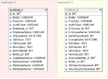
Figure 8: Fields of the audit trail from two applications

Figure 7 shows that there is quite a lot of overlap in what the different applications log. The basic information that is logged conforms with the specification as described in [2]. Apart from the basic information, the databases are extended with some application specific information. We think that the Aubittrail_B gives us more useful information then Audittrail_A. The Aubittrail_B trail logs information about ‗klant propositie‘ / customer propositions and ‗overeenkomst‘ / invoices. Based on that, we decided to take a data set of the audit trail from Application B as the input for our design. Due to legislations concerning privacy, we are not allowed to look into the actual database content and therefore we didn‘t analyze the audit trail any further than the database schema. For this research, a representative test set has been used. The test set contains two types of fields: obligatory fields, meaning every log record holds a value for that particular field, and optional fields, meaning that these fields can be empty or have NULL values.

4.3

Data warehouse Conversion

Based on the analysis of the available audit trail data test set, a data warehouse schema has to be defined. We have little knowledge and insight in the actual content of the data and the goal is to design a generic data warehouse which can handle any audit trail, the concept of labeling is introduced. The idea is based on annotated data provenance. Data provenance uses a form of labeling which adds meta information to data in order to group and relate data. By means of those labels, information gets meaning. Data then can be referred to via labels rather than actual content. As a result, the data warehouse has no knowledge of the data it holds, which means any log/data could be inserted into the data warehouse as long as the data warehouse schema for the audit log is conform certain guidelines.

34

always has the same characteristics. Based on these characteristics, the architecture, that will be designed on top of the data warehouse, can use the generic structure of the database.

4.3.1 Conversion rules and exceptions

To get a generic data warehouse, we are looking for rules to convert a log that is stored as a flat table in a database, to a normalized data warehouse.

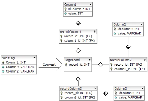
Initially, any log could be converted according to the known normalization algorithms[2]. By definition, the conversion produces a schema in the pattern as shown in Figure 9. The schema is an approved schema according to the normalization rules, but it is not an optimal solution. Every column of the log is placed in a separate table, and attached through a link table to the central LogRecord table. By introducing some exceptions, the schema produces a more optimal solution that still conforms to the normalization rules. The reason to add these exceptions is to decrease the database size and reduce the number of tables. The more tables, the slower the data warehouse becomes, since more joins are required.

When looking only at the column names, we see that some values are related and therefore should be stored together instead of in separate tables. We observed four main situations in which the data warehouse schema can be optimized without introducing new patterns in the schema.

 Exception 1: When the audit log contains a username and a field that already

uniquely identifies a user (e.g., user_id), those two columns could be combined instead of storing separately in two columns in the data warehouse. So the table

would become {user_id, username} instead of the default two columns

{user_id_id, user_id } and {username_id, username} with two link tables.

 Exception 2: When there are columns in the audit log which are related to each

other, such as, a ‗firstname‘ and a ‗lastname‘ column. Neither of the two uniquely identifies the other, but both are attributes of a person. Therefore these

fields should end up in the same table with a un