Mathematical programming approach to multidimensional mechanism design for single machine scheduling

MATHEMATICAL

PROGRAMMING APPROACH TO

MULTIDIMENSIONAL

MECHANISM DESIGN FOR

SINGLE MACHINE SCHEDULING

J. Duives

APPLIED MATHEMATICS

DISCRETE MATHEMATICS AND MATHEMATICAL PROGRAMMING EXAMINATION COMMITTEE

This master thesis is the result of my graduation project at the “Discrete Mathematics and Mathematical Programming (DMMP)” group of the Uni-versity of Twente. Using this opportunity, I would like to thank several people for their assistance, guidance and amusement during this project.

First of all many thanks go to Marc Uetz, my supervisor at the University of Twente. After a smooth cooperation during my internship, I happily accepted a graduation project under your “service”. Many times we have discussed and analysed problems we encountered for hours, possibly more than you intended to. I am grateful for this.

Furthermore I would like to thank all people who have made my gradua-tion project that more fun and easy going. For example, I really enjoyed the sometimes profound discussions with fellow students and professors during coffee breaks an during lunch. Moreover, I could always share my joy or disappointments with housemates, but also with friends from badminton or elsewhere.

Finally I would like to thank my family and girlfriend for their overall support. They helped and kept me motivated not only during my gradua-tion project, but also during the study preceding this thesis.

J. Duives.

Preface iii

1 Introduction 1

2 Optimal Mechanisms for Scheduling 5

2.1 Single Machine Scheduling Problem . . . 5

2.2 The 1-Dimensional Setting . . . 5

2.3 The 2-Dimensional Setting . . . 9

3 Mathematical Programming Formulations 13 3.1 Bayes-Nash Implementations . . . 14

3.2 Dominant Strategy Implementations . . . 15

3.3 Independence of Irrelevant Alternatives . . . 17

3.4 Implementation of MP Formulations . . . 18

4 Solution Method 20 4.1 Generating Instances . . . 20

4.2 Instance File Format . . . 22

4.3 Computational Procedure and Details . . . 22

5 Computational Results 26 5.1 Optimal Mechanisms and IIA . . . 26

5.2 BNIC-DSIC Equivalence . . . 30

6 Conclusion 37

7 Future Research 38

References 39

A Symbols and Abbreviations 42

B Instance File Format 44

C CPLEX LP file 45

1

Introduction

Mathematical optimization can be used to solve many economic problems concerning logistics and production. Collecting all information relevant for the problem, one can ‘simply’ select a solution optimizing a certain global objective from some set of available alternatives. However, quoting Kan-torovich [7], many of these classical optimization problems do not relate to realistic situations: “I want to emphasize again that the greater part of the problems of which I shall speak, relating to the organization and planning of production, are connected specially with the Soviet system of economy and in the majority of cases do not arise in the economy of a capitalist so-ciety”. Even more, “There [capitalism] the choice of output is determined not by the plan but by the interests and profits of individual capitalists”. Kantorovich is emphasising the fact that in capitalist economics, solving economic problems where certain decisions are left to individuals instead of a central authority, using classical optimization, is useless. For example, people may have a personal objective that induces a preference that does not match with the performance of the system as a whole. In those cases people might, based on their own and other peoples preferences, act strate-gically in order to manipulate the decision made by the central authority. Due to this strategic behaviour of individuals, classical optimization fails. The mathematical models to analyse such strategic situations are studied in Game Theory [12, 11].

In this thesis we consider a classical single machine scheduling problem. Given is a set of risk-neutral jobs that need to be processed non-preemptively on a single machine, that can handle only one job at a time. These jobs act selfishly as they all have a personal objective: to be processed as soon as

possible. Each job has a processing time pj and a disutility wj for waiting

one unit of time, which both can be private information. We refer to the private information of a job as its type. Although jobs do not known the actual type of other jobs, we assume that they do share common beliefs about other jobs’ types in terms of (discrete) probability distributions. An allocation rule, taking the role of central authority, assigns to each (possibly

untruthful) report of jobtypes, a scheduleσ, denoting the order in which the

jobs are processed on the machine. We assume that jobs’ preferences over

possible schedules are expressed as−wjSj(σ), whereSj(σ) is the start time

of jobj in scheduleσ.

Depending on their disutility for waiting, jobs are compensated for wait-ing in the form of a payment. In this settwait-ing a mechanisms consists of an allocation rule and a payment scheme, defining the payments jobs receive to be compensated for waiting. The payments influence the objectives of

jobs as follows. Let us denote the utility of jobj when scheduleσ is chosen

and it receives paymentπj, byπj−wjSj(σ), referred to in the literature as

quasi-linear utility with respect to payment πj [9]1. We assume that jobs

seek to optimize their (expected) utility. We only consider direct revela-tion mechanisms, that is, mechanisms in which the only decision made by jobs, is the report of their type. Even more, by making use of Myersons’ famous revelation principle [10], we may restrict ourselves to truthful or in-centive compatible mechanisms, which are mechanisms where jobs have the incentive to report their type truthfully. More specific, Bayes-Nash incentive compatible (BNIC) mechanisms motivate jobs to report truthfully, provided that other jobs also do so, whereas (stronger) dominant strategy incentive compatible (DSIC) mechanisms motivate jobs to report truthfully regardless of what other jobs do. In this setting our goal is to find mechanisms that minimize the expected total payment made to the jobs, while motivating jobs to report their weight truthfully (either BNIC or DSIC).

This problem, mainly the special case of 1-dimensional types (public

processing times pj and privatewj), has been considered earlier in a paper

by Heydenreich et al. [5]. They prove that serving jobs in order of

non-increasing ratio of modified weights over processing times, ¯wj/pj, is optimal

1

[10], i.e. minimizes the payments made to the jobs while being Bayes-Nash incentive compatible. Moreover, Heydenreich et al. [6] prove that Bayes-Nash incentive compatibility and dominant strategy incentive compatibility is equivalent in the sense that if there exists a mechanism that is Bayes-Nash incentive compatible, then there exists a dominant strategy incentive compatible with the same expected total payment. Finally, in search for a closed formula for the optimal mechanism also in the 2-dimensional setting

(bothpj andwj private), Heydenreich et al. [5] propose an example to show

that optimal mechanisms in the 2-dimensional setting in general do not satisfy a condition called IIA, independence of irrelevant alternatives. This example gives a hind towards intractability of the 2-dimensional mechanism design problem. However, that example was flawed.

Motivated by the questions left open in [5], in this thesis we are inter-ested in getting more insight into properties of (optimal) mechanisms for the 2-dimensional setting. In particular, we are interested in the IIA condition, the minimal condition that an optimal mechanism should have if a closed formula were to exist. Constructing a new example by hand to prove that optimal mechanisms in the 2-dimensional setting in general do not satisfy IIA, turned out to be difficult and time consuming. Therefore we decided to switch to a more systematic approach, i.e. optimal mechanism design by mathematical programming, also known as automated mechanism design [2, 13]. In automated mechanism design the mechanism is designed ‘auto-matically’ for the setting and objective at hand, where automatically refers to the use of IP solvers.

In the flavour of recent work on automated mechanism design as pro-posed by Conitzer and Sandholm [2, 13], we formulate the optimal mecha-nism design problem for this scheduling application as Mixed Integer Linear Programming Problem (MIP). This MIP formulation allows us, using ILOG CPLEX as solver for the MIPs, to compare optimal solutions for different types of mechanisms in the scheduling problem. Indeed, by this approach we are able to reconfirm that optimal mechanisms in the 2-dimensional set-ting in general do not satisfy IIA, reconfirming a theorem formulated in [5]. Additionally we use this MIP to prove that for the 2-dimensional setting, BNIC and DSIC are in general not equivalent in the sense that there is an instance where the minimal expected total payments achieved by the DSIC mechanism exceed those of the optimal Bayes-Nash mechanism. Besides these general results, we compare different types of mechanisms in specific types of instances to possibly strengthen our findings.

2

Optimal Mechanisms for Scheduling

In this section we start by discussing the non-strategic version of the single machine scheduling problem. Then we switch to the strategic single ma-chine scheduling problem. First we discuss the 1-dimensional setting for this problem as well as some results by Heydenreich et al [5]. Even more, we elaborate on some related results by Manelli and Vincent [8] and Ger-shkov et al. [4]. Eventually we switch to the 2-dimensional single machine scheduling problem together with the flawed counterexample that formed the starting point for our research.

2.1 Single Machine Scheduling Problem

Let us consider the standard single machine scheduling problem. Given is a

set of jobsJ ={1, . . . , n}, which have to be processed non-preemptively on a

single machine that can handle one job at a time. Each jobjhas a processing

time pj and a disutility for waiting one unit of time, also called its weight

wj, both publicly known. Let S = {σ|σ is a permutation of (1,. . . ,n)} be

the set of feasible schedules, i.e. the order in which jobs are processed on the

machine. Denoting by σj the position of job j in schedule σ, the start or

waiting time of job jis represented bySj(σ) =Pσk<σjpk. Note that we do

not assume idle time, i.e. jobs are processed immediately after one another. In this setting, all decisions are made by a central authority, e.g. sched-uler, who chooses an order in which to process the jobs and we do not need to account for strategic behaviour of jobs. One of the standard objectives for this problem is to minimize the sum of weighted completion times, or equivalently, minimize the sum of weighted start times. Note that the latter is identical to the total disutility for waiting. This standard objective is optimized by a well known list scheduling algorithm known as Smith’s rule [14], i.e. scheduling jobs in order of non-increasing ratio of weight over

pro-cessing time wj/pj. From this standard single machine scheduling problem

we switch to the strategic version of this problem, which we consider in the remainder of this thesis.

2.2 The 1-Dimensional Setting

A first departure from the non-strategic setting is that in the strategic setting we have a set of selfish jobs that act strategically. For the 1-dimensional

whereaswj, the weight of jobj, is private information2. Although the weight of a job is private information, other jobs share common beliefs about jobs’

types in terms of probability distributions. Let Wj = {wj1, . . . , w

mj

j }

de-note the set of possible weights of jobj. The corresponding (finite discrete)

probability distribution isφj and φj(wj) denotes the probability associated

with wj. Both Wj and φj are public information. The set of all type

profiles is denoted byW = Πj∈JWj and φis the joint probability

distribu-tion of w = (w1, . . . , wn) ∈ W, i.e. φ(w) = Πjφj(wj). For each job j, let

W−j = Πk6=jWk, let w−j ∈ W−j and let φ−j be the corresponding

proba-bility distribution. Note that (wj, w−j) is the type profile where job j has

typewj and the types of all other jobs are w−j.f

In this setting, a mechanism consists of an allocation rulef and a

pay-ment scheme π. We consider only direct revelation mechanisms, which are

mechanisms in which the only decision made by jobs, is the report of their

type. For the remainder of this thesis we denote by wj a job’s true weight

and we denote by ˜wj the reported weight of a job, which may be both true

and false. Letw−j and ˜w−j be defined analogously. Based on the reported

types, an allocation rule f, taking the role of central authority, chooses a

scheduleσ. In other words, the allocation rule is a mapping from the set of

type profiles to the set of schedules, that is f :W → S. Job j is

compen-sated for its waiting time by paymentπj, assigned by the payment scheme

π. To express the appreciation of a job for a certain schedule and payment

scheme we have to introduce some extra notations. Given job j’s waiting

timeSj and its weightwj, it encounters a valuation of−wjSj(σ) for schedule

σ. This means the earlier the better, with a cost of wj per one unit of time.

Additionally receiving a paymentπj, its utility is expressed byπj−wjSj(σ),

i.e. we assume what is called quasi-linear utility [9]. Denote by

ESj(f,w˜j) :=

X

w−j∈W−j

Sj(f( ˜wj, w−j))φ−j(w−j)

the expected waiting time of jobjif it reports weight ˜wjand allocation rulef

is applied. Note thatf( ˜wj,w˜−j) =σand therefore we writeSj(f( ˜wj,w˜−j)) =

2

Sj(σ). Let3

Eπj( ˜wj) :=

X

w−j∈W−j

πj( ˜wj, w−j)φ−j(w−j)

be the expected payment to job j if it reports weight ˜wj.

Definition 1. A mechanism (f, π) is incentive compatible if jobs have the incentive to report their weight truthfully, i.e. a job obtains highest utility by reporting its true weight. More specifically, a mechanism is:

• dominant strategy incentive compatible (DSIC) if for every job j and

every two types wj,w˜j ∈Wj, and any report w˜−j of other jobs, πj(wj,w˜−j)−wjSj(f(wj,w˜−j))≥πj( ˜wj,w˜−j)−wjSj(f( ˜wj,w˜−j)).

(2.1)

If for allocation rule f there exists a payment scheme π such that

(f, π) is DSIC, then f is called implementable in dominant strategies.

The payment scheme π is referred to as a dominant strategy incentive

compatible payment scheme.

• Bayes-Nash incentive compatible (BNIC) if for every job j and every

two types wj,w˜j ∈Wj, under the assumption that all jobs apart from

j report truthfully,

Eπj(wj)−wjESj(f, wj)≥Eπj( ˜wj)−wjESj(f,w˜j). (2.2)

If for allocation rulef there exists a payment schemeπsuch that(f, π)

is BNIC, then f is called Bayes-Nash implementable. The payment

schemeπis referred to as an Bayes-Nash incentive compatible payment

scheme.

Our definition requires jobs to be truthful instead of playing other strate-gies. This however, is no loss of generality by Myersons’ revelation principle [10], as incentive compatible, direct revelation mechanisms can be designed

to achieve the same equilibrium payment of any other mechanism4. Note

3

Note that we defineESj(f,wj) and˜ Eπj( ˜wj) only for true reports of jobs other than jobj. We only need these definitions in a setting where all other jobs report truthfully, as we only consider solutions where truthful reports are an equilibrium. To defineESj(f,wj)˜ and Eπj( ˜wj) more generally, would require to take the probability distributions for un-truthful reports of ˜w−jof other agents into account.

4_{The proof for the revelation principle for direct revelation mechanisms is as follows.}

Let us denote by sj the strategy of job j, i.e. sj(wj) is the weight job j reports, given his true weight wj. Now we can turn any direct revelation mechanism with equilibrium s= (s1, . . . , sn) and allocation rulegin an incentive compatible mechanism, by defining

allocation rule f(t1, . . . , tn) = g(s1(t1), . . . , sn(tn)), i.e. allocation rulef =g◦s simply

that dominant strategy incentive compatibility is the strongest equilibrium

one can ask for. Regardless ofw−j, the report of other jobs, reporting its true

type is optimal for every job. Bayes-Nash incentive compatibility is a weaker condition and is trivially implied by dominant strategy incentive compati-bility. Intuitively, it says the following: given that jobs are risk-neutral and

that all jobs apart from jobjreport truthfully, taking expectations over the

possible type profiles of other jobs, it is optimal for jobjto report its weight

truthfully.

Moreover, rationality of jobs participating in the game is expressed by the following definition.

Definition 2. A dominant strategy incentive compatible mechanism (f, π)

is individually rational (IR) if for every jobj, every true type wj ∈Wj and

any report w˜−j of other jobs,

πj(wj,w˜−j)−wjSj(f(wj,w˜−j))≥0. (2.3)

In other words, individual rationality for DSIC mechanisms implies that the utility of a job reporting its true weight should be positive, regardless what other jobs report. For BNIC mechanisms we have a slightly different definition.

Definition 3. A Bayes-Nash incentive compatible mechanism (f, π) is

in-dividually rational (IRE) if for every jobj and every true type wj ∈Wj,

Eπj(wj)−wjESj(f, wj)≥0. (2.4)

For BNIC mechanisms rationality implies that the expected utility of a job reporting its true weight should be positive. Note that we speak of BNIC mechanisms and therefore the reports of other jobs are assumed to be truthful.

In [5], Heydenreich et al. consider for the scheduling problem so far intro-duced here, the minimal expected total payment made to the jobs achieved by an allocation rule. For the DSIC setting we assume jobs to maximize their utility, whereas for the DSIC setting we assume jobs to maximize their expected utility.

Definition 4. An optimal mechanisms(f, π)is a mechanism that is Bayes-Nash incentive compatible, individually rational and minimizes the expected

total payment made to jobs. Allocation rulef is called an optimal allocation

Heydenreich et al. [5] give an explicit formula for the optimal mechanism

in the 1-dimensional setting5. The optimal allocation rule f is a

modifica-tion of Smith’s rule. Ergo, for the 1-dimensional scheduling problem the optimal allocation rule is rather simple; scheduling jobs in non-increasing order of weight over processing time ratios, using certain modified weights. Important to mention is that both the modified weights and the payment to a job can be computed using only the characteristics (type and distribu-tion) of the job itself. Furthermore Heydenreich et al. [6] prove that for the 1-dimensional scheduling problem at hand BNIC and DSIC mechanisms in some sense are equivalent. They show there exists a mechanism that is dom-inant strategy incentive compatible and individually rational, and achieves the same expected total payment as the optimal mechanism defined above. Manelli and Vincent [8] obtain a similar result for single item auctions with what they refer to as linear utilities. They investigate the model in which a single indivisible object is divided among finitely many agents. The valuation of the agents for the object is private information, although as in our case, from each agent’s viewpoint, those valuations are independently distributed according to known distributions. They prove that for this set-ting, there exists a mechanism that is Bayes-Nash incentive compatible if and only if there exists a dominant strategy incentive compatible mecha-nism that generates the same expected payments and utilities. For general settings with linear utility and 1-dimensional types Gershkov et al. [4] prove that in settings with only two possible outcomes, e.g. two schedules, BNIC and DSIC is equivalent. However, they also show by counterexample that such an BNIC-DSIC equivalence can only be valid in restrictive environ-ments, as in general, BNIC and DSIC are not equivalent as soon as there are at least three possible outcomes.

2.3 The 2-Dimensional Setting

Having analysed the 1-dimensional setting of the scheduling problem, ques-tions arise whether the results from Heydenreich et al. hold for a setting where both the weight and the processing time of a job are private

infor-mation. Analogously to the 1-dimensional case, the processing time of job j

is some element from the set Pj ={p1j, . . . , p

qj

j }. For the 2-dimensional

set-ting,tj, the type of jobj is a combination of its weight and processing time

and is denoted by (wj, pj). The types are drawn from the set Wj×Pj, the

type space of job j, also denoted by Tj, according to some publicly known

probability distribution φj. Then φj(wj, pj) is the probability associated

with type (wj, pj). As for the 1-dimensional setting we will denote by tj

and pj job j’s true type and processing time respectively, whereas reports

˜

tj and ˜pj can be both true and false. The set of all type profiles we denote

byT = Πj∈J(Wj×Pj) andT−j = Πr6=j(Wr×Pr) is the set of type profiles

of all jobs except job j. We denote by φthe joint probability distribution

of t = (w1, p1, . . . , wn, pn) ∈T, ergo φ(t) = Πjφj(wj, pj). Let t−j and φ−j be defined analogously. Redefining the type of a job, the expressions for the expected start time and payment to a job also slightly change. Denote by

ESj(f,w˜j,p˜j) :=

X

t−j∈T−j

Sj(f(( ˜wj,p˜j), t−j))φ−j(t−j)

the expected start time of jobj when it reports type ( ˜wj,p˜j) and allocation

rulef is applied. And let6

Eπj( ˜wj,p˜j) :=

X

t−j∈T−j

πj(( ˜wj,p˜j), t−j)φ−j(t−j)

be the expected payment to job j when it reports type ( ˜wj,p˜j). Now the

processing time of a job is private information too, jobs have to report both their weight and processing time. Whereas for their weight, jobs could over-and understate it, we make the following assumption on a jobs possible report of its processing time.

Assumption 1. We assume that jobs can only overstate their processing time, that is, jobs can only report a larger processing time then their true processing time.

This assumption is made, since reporting a lower processing time than its true processing time can easily be punished by pre-empting the job early (after the reported time). Note that by regarding the processing time of a job as private information, the valuation of a job for a schedule does now also depend on private information of other jobs, namely the processing time

of jobs that are scheduled before jobj.

For the 2-dimensional setting also the definitions of BNIC and DSIC change.

Definition 5. A mechanism(f, π) is:

6

• dominant strategy incentive compatible if for every jobjand every two types (wj, pj),( ˜wj,p˜j) ∈ Tj such that pj ≤ p˜j, and any report ˜t−j of

other jobs,

πj((wj, pj),˜t−j)−wjSj(f((wj, pj),˜t−j))≥

πj(( ˜wj,p˜j),˜t−j)−wjSj(f( ˜wj,p˜j),t˜−j)). (2.5)

• Bayes-Nash incentive compatible if for every job j and every two types

(wj, pj),( ˜wj,p˜j)∈Tj such that pj ≤p˜j, under the assumption that all

jobs apart from j report truthfully,

Eπj(wj, pj)−wjESj(f, wj, pj)≥

Eπj( ˜wj,p˜j)−wjESj(f,w˜j,p˜j). (2.6)

Note that as for the 1-dimensional setting this definition requires jobs to be truthful instead of playing other strategies. Furthermore also for the 2-dimensional setting, Bayes-Nash incentive compatibility is trivially implied by dominant strategy incentive compatibility. The definition for individual rationality for a DSIC or BNIC mechanism for the 2-dimensional setting read as follows.

Definition 6. A dominant strategy incentive compatible mechanism (f, π)

is individually rational (IR) if for every job j, every true (wj, pj)∈Tj and

any report t˜−j of other jobs,

πj((wj, pj),˜t−j)−wjSj(f((wj, pj),˜t−j))≥0. (2.7)

Definition 7. A Bayes-Nash incentive compatible mechanism (f, π) is in-dividually rational (IRE) if for every job jand every true type(wj, pj)∈Tj,

Eπj(wj, pj)−wjESj(f, wj, pj)≥0. (2.8)

As for the 1-dimensional setting we seek to find the minimal expected

total payment made to the jobs achieved by an allocation rule. Letf be an

allocation rule, then we denote byEπf_{(·) a payment scheme that minimizes}

the expected total payment made to the jobs among all payment schemes

that makef Bayes-Nash implementable and IRE. ThenEπf(˜tj) denotes the

payment to agent j declaring type ˜tj under payment scheme Eπf.

Analo-gously, we denote by πf(·) a payment scheme that minimizes the expected

total payment made to the jobs among all payment schemes that make f

payment to agentj declaring type ˜tj and given the report of types of other

jobs ˜t−j, under πf. Finally EPmin(f) andPmin(f) denote the

correspond-ing minimal expected total payments made to the jobs, achieved by payment

schemeEπf andπf respectively. Analogously to the 1-dimensional setting,

an optimal mechanism is a mechanism that is Bayes-Nash incentive compat-ible, individually rational and minimizes the expected total payment made

EPmin(f) to jobs.

As a matter of fact, optimal mechanisms for the 2-dimensional setting do not seem to have a simple characterisation as in the 1-dimensional setting. In order to give a hint towards the intractability of the 2-dimensional optimal mechanism design problem, Heydenreich et al. [5] give an example to show that the optimal mechanism does not in general satisfy a condition known as IIA.

Definition 8. We say that an allocation rule f satisfies independence of

irrelevant alternatives (IIA) if the relative order7 of any two jobs j1 and

j2 is the same in the schedules f( ˜t1) and f( ˜t2) for any two type profiles ˜

t1,t˜2∈T that differ only in the types of jobs from J\ {j1, j2}.

In other words, an allocation rulef satisfies IIA if the relative order of

two jobs is independent of all other jobs. Heydenreich et al. try to show by counterexample that the optimal allocation rule for the 2-dimensional setting does in general not satisfy IIA. In [5] they suggest an instance with three jobs, where the minimal expected payments achieved by an allocation rule that is IIA, exceed the minimal expected payments achieved by an allocation rule that does not satisfy the IIA condition. However, this example was flawed.

The equivalence of BNIC and DSIC for the 2-dimensional setting has not been analysed by Heydenreich et al. and will be discussed in the remainder of this thesis, together with the search for a new example regarding the IIA property of optimal mechanisms.

7

The relative order of two jobsj1 andj2 in a schedule is the position of jobj1 relative

3

Mathematical Programming Formulations

In Section 2 we discussed a single machine scheduling problem that was analysed by Heydenreich et al. The driving questions behind our research have been getting more insight into optimal mechanisms, as well as trying to prove or disprove BNIC-DSIC equivalence for the 2-dimensional setting

of this problem. As both questions have been attacked using the same

approach, we will first give a detailed description of our approach, where we will later come back to the results.

The initial direction of our research was to find a new instance to prove that the optimal allocation rule for the 2-dimensional setting does in general not satisfy the IIA condition. This would give a hint towards intractability of the optimal mechanism design problem. Creating and checking an instance by hand turned out to be rather difficult and time consuming. Therefore we decided to use a mathematical programming approach, a more systematic approach that has recently become known as automated mechanism design. In the words of Conitzer and Sandholm [2, 13], in automated mechanism design “the mechanism is computationally created for the specific prob-lem instance at hand”. An advantage of automated mechanism design over (manual) mechanism design is that it easily can be used in settings beyond those that have been studied using (manual) mechanism design. Further-more it may yield better mechanisms because the mechanisms are tailored to the specific setting. A disadvantage is that the optimal mechanism design problem has to be solved anew for every instance.

Applying the concept of automated mechanism design we model and solve the optimal mechanism design problem for the 2-dimensional setting by formulating the problem as a mathematical program (MP), to be pre-cise a mixed integer (quadratically constrained) program (MI(QC)P). This allows us to compare different types of mechanisms. Given an instance, the

input for the mixed integer program consists of a set of jobs j ∈ {1, . . . , n}

with associated typestj = (wj, pj)∈Tj and probabilities φj(tj) for typetj,

as defined in Section 2. We enumerate type profilest= (t1, . . . , tn) with

cor-responding probability distribution φ(t) as well as schedules σ, from which

follows σi, the position of jobiin scheduleσ. Having defined these

param-eters we can calculate Stσj, the start or waiting time of job j in scheduleσ

while the type profile is t. In addition, we introduce binary variables

xtσ =

1 if scheduleσ is assigned to type profilet

0 otherwise

pre-cisely encode the allocation rule of the desired mechanism. Furthermore for

the BNIC setting we introduce continuous variables Eπj(tj) and ESj(tj)

representing the expected payment to and the expected start time of job

j, reporting type tj respectively. For the DSIC setting we only introduce

continuous variablesπtσj representing the payment to jobj given the

over-all type profile t and schedule σ. A solution of the integer program is an

allocation rule, together with a corresponding payment scheme.

3.1 Bayes-Nash Implementations

The problem of finding an optimal mechanism, i.e. a mechanism that is Bayes-Nash incentive compatible, individually rational and among such mech-anisms minimizes the expected total payments that have to be made to the jobs, can be represented by the following mixed integer program.

minX

j

X

tj

φj(tj)Eπj(tj) (3.1a)

X

σ

xtσ= 1 ∀t (3.1b)

ESj(tj) =

X

t−j,σ

Stσjxtσφ−j(t−j) ∀j, tj (3.1c)

Eπj(tj)≥wj(tj)ESj(tj) ∀j, tj (3.1d)

Eπj(tij)≥Eπj(tkj)

−wj(tij)

ESj(tkj)−ESj(tij)

∀j,(ti_j, tk_j)∈Tbn (3.1e)

xtσ∈ {0,1} (3.1f)

Eπj, ESj ≥0 (3.1g)

Continuous variables Eπj(tj) denote the expected payment to job j

hav-ing type tj, as defined in Section 2.3. Together they define the payment

scheme of the Bayes-Nash incentive compatible optimal mechanism. Objec-tive (3.1a) minimizes the expected total payments made to all jobs, whereas constraints (3.1b) enforce a feasible allocation rule by assigning exactly one

schedule to each type profile. Note that the notation ofESj(tj), the variable

for the expected start time of a job, is slightly different from the notation in Section 2.3. In Section 2.3 the expected start time was explicitly defined

only for allocation rule f and type tj, where the same result is now

ob-tained in (3.1c) by summing also over all schedules σ and multiplying by

The individual rationality and incentive constraints are represented by

(3.1d) and (3.1e) respectively, although the latter are somewhat rearranged8.

According to Definition 5 the incentive constraints only hold for pairs of

(ti_j, tk_j) for which processing time of jobj having typeti_j, is smaller or equal

to processing time of job j having type tk_j, as jobs cannot overstate their

processing time. This is implemented by defining constraints (3.1e) only for (ti_j, tk_j)∈Tbn where

Tbn={(ti_j, tk_j)|pj(tij)≤pj(tkj)}.

Finally constraints (3.1f) express the integrality of thextσvariables and

con-straints (3.1g) express the bounds on the expected payment to and expected

start time of job j.

3.2 Dominant Strategy Implementations

To compare BNIC and DSIC mechanisms, we build a mathematical program for the DSIC setting, too. The problem of finding a mechanism that is dominant strategy incentive compatible, individually rational and among such mechanisms minimizes the expected total payments that have to be made to the jobs, can be represented by the following mixed integer program.

minX

t

X

σ

X

j

φ(t)πtσj (3.2a)

X

σ

xtσ= 1 ∀t (3.2b)

πtσj ≥wj(t)Stσjxtσ ∀t, σ, j (3.2c)

πtσj ≥πt0_σ0_j −wj(t)(S_t0_σ0_j−S_tσj)

+M(xtσ−1) ∀σ, σ0, j,(t, t0)∈Tds (3.2d)

xtσ∈ {0,1} (3.2e)

πtσj ≥0 (3.2f)

Note that this MIP is very similar to the one discussed in Section 3.1. There are however some important dissimilarities concerning the variables and the individual rationality and incentive constraints. In (3.2), the variables for

the expected payments are replaced by variables πtσj, representing the

pay-ment to job j given the overall type profile t and schedule σ. As we still

seek to minimize the expected total payments made to the jobs, the objec-tive is represented by (3.2a). Intuiobjec-tively one would say that we only need to

define payments for all type profilestand jobsj, as ultimately to each type

profile will be assigned only one schedule σ. However, up front we do not

know which schedule is assigned to which type profile and therefore we also

have to introduce payments for all schedulesσ. The constraints that enforce

a feasible allocation rule remain unchanged and are represented by (3.2b). In the DSIC setting we no longer need expected start times and therefore constraints (3.1c) can be omitted and the individual rationality constraints

translate to (3.2c). These constraints9 are stronger than constraints (3.1d),

as individual rationality has to hold not only in expectation, but for every type profile - schedule combination that is chosen by the allocation rule.

In addition to changing the start time and payment variables, we have to introduce a big-M construction for the rearranged incentive constraints (3.2d). This is to enforce that the incentive constraints are tight for type profile - schedule combinations that are chosen by the allocation rule and are

trivially fulfilled otherwise10. As for the BNIC setting jobs cannot overstate

their processing time, constraints (3.2d) only hold for pairs of type profiles

(t, t0) such that the processing time of job j under type profile t is smaller

or equal than its processing time under type profile t0. Also the reported

types of other jobs must be equal in both t and t0. Even more, when the

type profiles are identical, the incentive constraints in combination with the

MP are fulfilled trivially, hence we do not define them when t = t0. A

schematic representation ofTds, the set for which the incentive constraints

are defined, can be found in Table 1. In this table +, −and +−represent

that the corresponding condition is fulfilled, not fulfilled or either of both, respectively. Note that for type profile-schedule combinations not chosen by the allocation rule, both constraints (3.2c) and (3.2d) are trivially fulfilled. Therefore, for these combinations, the payments are automatically set to 0

due to the minimizing objective and for each t we are left with only one σ

for whichπtσj >0. Finally constraints (3.2e) express the integrality of the

xtσ variables and constraints (3.2f) express the bounds on the payment to

jobj when the type profile is tand schedule σ is chosen.

9

Note that we introducewj(t), representing the weight of jobj when the overall type profile ist.

10

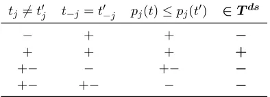
tj6=t0j t−j=t−0 j pj(t)≤pj(t0) ∈Tds

− + + −

+ + + +

+− − +− −

+− +− − −

Table 1: Schematic representation of Tds, the set of type profile pairs for which the dominant strategy incentive constraints are defined.

3.3 Independence of Irrelevant Alternatives

Using mathematical programs (3.1) and (3.2) we can compare BNIC and DSIC mechanisms. However, to check whether the optimal allocation rule does in general satisfy IIA, we must be able to add constraints to MIP

(3.1) that imply the IIA condition11. By adding the following quadratic

constraints

xtσxt0_σ0 ≤(σ_j−σi)(σ0_j−σ0_i)x_tσx_t0_σ0 ∀(t, t0)∈Tiia, σ, σ0, j, i6=j (3.3)

to the mathematical formulation of the Bayes-Nash optimal mechanism de-sign problem, the solution of the modified program is an allocation rule that

satisfies IIA, together with a corresponding payment scheme12.

The constraints are based on the fact that if the relative order of job

j and job i in schedule σ and σ0 is different, i.e. (σj −σi)(σ0j −σ0i) < 0,

then not both xtσ and xt0_σ0 can equal 1. However, we must pay attention

for which pairs (t, t0) we define the IIA constraints. By definition of IIA we

are interested only in pairs (t, t0) that differ only in the types of jobs from

J \ {i, j}, so tj = t0j and ti = t0i. Furthermore, if also t = t

0_{, constraints}

(3.3) in combination with the MIP are fulfilled trivially and therefore we

only define the IIA constraints for t6= t0. The set of pairs (t, t0) that have

these properties we denote by Tiia. A schematic representationTiia can be

found in Table 2. But even more, if i =j we would set either xtσ = 0 or

xt0_σ0 = 0, although the relative order of the jobj and job iis identical and

11_{Not to by adding the IIA constraints to MIP (3.2), one might also try to (dis)prove}

that the allocation rule that is implementable in dominant strategies and minimizes the total expected payments made to jobs, satisfies the IIA condition. However, that is behind the scope of this thesis.

12

After the research was finished, we found out that the same result can be retrieved by adding constraintsxtσ+xt0_σ0 ≤1 for the samet, t0, σ, σ0, j, i. This substitution leads to a

we would make the MP infeasible. Therefore the IIA constraints are defined

only when (t, t0) ∈ Tiia and i 6= j. Finally note that by adding the IIA

constraints to MIP (3.1), the MIP changes to a mixed integer quadratically constraint program (MIQCP).

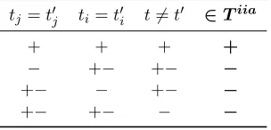
tj=t0j ti=t0i t6=t0 ∈Tiia

+ + + +

− +− +− −

+− − +− −

+− +− − −

Table 2: Schematic representation of Tiia, the set of type profile pairs for which the IIA constraints are defined.

3.4 Implementation of MP Formulations

The MIPs and MIQCPs proposed in the previous section are solved using ILOG CPLEX. This is a tool for solving several kinds of mathematical op-timization problems, among them MIPs and MIQCPs. It is folklore that reformulating constraints or even the complete mathematical program can have a substantial influence on the solving time of the MP, therefore we seek to ‘massage’ the MPs in order to minimize the solving time. One can think of adding or removing constraints and eliminating variables. At default settings, ILOG CPLEX uses several techniques to preprocess problems by simplifying constraints, reducing problem size, and eliminating redundancy and symmetry. However, these techniques can be seen as a black-box and therefore we additionally tried to modify the MPs ourself to improve the solving time.

One of the most obvious modifications is to get rid of quadratic con-straints (3.3). There are several ways to linearise these concon-straints and we

use a very basic one. We replace all products xtσxt0_σ0 in the program by

binary variablesytσt0_σ0, so that we obtain

ytσt0_σ0 ≤(σ_j−σi)(σ_j0 −σ_i0)y_tσt0_σ0 ∀(t, t0)∈Tiia, σ, σ0, j, i6=j (3.4)

as new IIA constraints. To assure that the variablesytσt0_σ0 attain the same

con-straints.

ytσt0_σ0 ≤x_tσ ∀t, σ, t0, σ0 (3.5a)

ytσt0_σ0 ≤x_t0_σ0 ∀t, σ, t0, σ0 (3.5b)

ytσt0_σ0 ≥x_tσ+x_t0_σ0 −1 ∀t, σ, t0, σ0 (3.5c)

We can define the ytσt0_σ0 variables for all t,σ,t0 and σ0 as in (3.5). However,

we only need them to replace all xtσxt0_σ0 products occurring in the MP.

Therefore we define theyvariables and corresponding constraints (3.5) only

fort and t0 for which (t, t0)∈Tiia.

In constraints (3.3) there is a lot of symmetry since xtσxt0_σ0 =x_t0_σ0x_tσ.

Replacing these quadratic constraints by introducing y variables, the

sym-metry remains (ytσt0_σ0 = y_t0_σ0_tσ). To get rid of this symmetry, we define

both the quadratic and linearised IIA constraints as well as the y variables

and constraints (3.5) only for t, σ, t0, σ0 such that t· |S|+σ < t0· |S|+σ0,

assuming that the types and schedules are ordered in some arbitrary way. This way, we reduce the number of variables and constraints by roughly a

factor two. Note that we do not define them when t· |S|+σ=t0· |S|+σ0,

as this implies thatt=t0, hence (t, t0)∈/ Tiia.

With our last modification we can even further reduce the number of

IIA constraints. Let us consider the value of (σj−σi)(σ0j−σi0) for different

σ, σ0, i, j. At this point for all cases where (σj −σi)(σ0j −σi0) 6= 0 the IIA

constraints are defined. However, (σj −σi)(σj0 − σ0i) > 0 implies (σj −

σi)(σ0j −σi0) ≥ 1 as σi is integer and in this case the IIA constraints are

redundant. Therefore we need to define constraints (3.3) and (3.4) only for (σj−σi)(σj0 −σ

0

4

Solution Method

In the previous section we formulated mathematical programs for different types of mechanisms in the 2-dimensional scheduling problem. In this section we give an extensive description of the method we use to compare BNIC and DSIC mechanism, fulfilling the IIA constraints or not, whereas the computational results themselves can be found in Section 5.

First we systematically generate instances at random, which we use for our research. Then we construct, using the instances, the proper mathe-matical programs and finally we optimally solve the MPs to find answers to our research questions mentioned in Section 3. All components have been realized in a program written in C++, which successively executes the components, one by one described in this section.

4.1 Generating Instances

Our first step is to generate instances, which are necessary to test our hy-potheses on. The size of the instances we generate depends on the research question we focus on. As the definition of IIA is irrelevant for instances with one or two jobs, for this part of the research we only generate instances with three or more jobs. To investigate similarities between BNIC and DSIC we also generate instances with two jobs. We do not want the solving time of the MPs to be too long and therefore we initially focus on smaller instances. If we do not find any results using these instances we subsequently increase the number of jobs and/or types of a job.

The input arguments of the C++ program consist of the number of jobs and if desired the number of types per job. One can also decide to generate instances with a random number of jobs or types per job. Given the number of jobs and types per job, the program generates for each type of a job a corresponding weight, processing time and probability.

The weights and processing times of a job chosen first, are chosen

uni-formly over the discrete integer set{1, . . . ,10}. However, to ensure that we

do not encounter equal weights or processing times for a job, we iteratively generate a weight or processing time and delete its value from the set from which we chose the last value. From the new set we obtain, we again se-lect uniformly a new weight or processing time. We will denote this type of distribution by (discrete, ‘uniform’). The probabilities of the types of a job cannot be chosen randomly over a discrete set, as the sum over the

probabilities of the types of a job must be equal to 1. Instead, per jobj, for

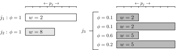
Figure 1: Graphical representation of instance in Appendix B.

set {0, . . . ,100}. Afterwards we divide the selected numbers vi_j by P

ivji,

the sum of all numbers chosen for the jobtypes of job j. This leaves us

with probabilities φj(tj), which all have the same expected value. However,

eventually we only need instances with probabilities rounded to one-tenths or one-hundredths. Therefore we round down all probabilities except for the

last one, which we set to the remaining probability13. We will denote the

obtained distribution by (discrete, E(tj) ≈ E(t0j)). Note that initially we

use probabilities rounded to one-tenths, whereas we round the probabilities to one-hundredths if we do not obtain results with the former. An overview of the type, range and distribution of the elements of a job’s type can be found in Table 3.

Property Symbol Type Range Distribution

Weight wj Integer [1,10] Discrete ‘uniform’

Processing time pj Integer [1,10] Discrete ‘uniform’

Probability type φj(tj) Decimal [0.0,1.0] Discrete, E(tj)≈E(t0j)

Probability type φj(tj) Hundredths [0.00,1.00] Discrete, E(tj)≈E(t0j)

Table 3: Type, range and distribution of the elements of a type of a job.

To select ‘random’ numbers from some discrete set, we use the rand()

function in C++. This is a pseudo-random integral number generator con-taining an algorithm that returns a sequence of apparently non-related num-bers each time it is called. The algorithm uses a seed to generate the series,

which should be initialized to some distinctive value using srand().

Choos-ing the same seed value will lead to the same ‘random’ sequence and thus makes it possible to reproduce the experiments any time. An example of an instance we generate for our research is sketched in Figure 1.

Once proven or disproven that optimal mechanisms do in general satisfy

the IIA condition, or that BNIC and DSIC in general is equivalent, we seek to specify our general results. To test our results on more specific instances, we therefore generate instances with specific properties. One type of instances we investigate are instances for which the types of job have a product distribution.

Definition 9. A product distribution is a probability distribution of which the marginal distributions are pairwise stochastically independent.

In the 2-dimensional scheduling problem the pair (wj, pj) equals tj, the

type of job j. Suppose that the weight and processing time of job j have

probability distributionϕj and ψj respectively14. Then φj, the probability

distribution associated with typetj, is a product distribution if for all wj ∈

Wj and pj ∈Pj holds φj(wj, pj) = ϕj(wj)·ψj(pj). In other words, φj is a

product distribution if the probability associated with having type (wj, pj)

is the product of the marginal distributions ϕ and ψ for having weight wj

and processing time pj, respectively.

4.2 Instance File Format

The information of an instance is written to a text file in a specific format. The first line contains only the number of jobs, whereas the second line contains the number of types per job, separated by a white space. The remainder of the text file consists of a single line for each type, the types sorted per job, in ascending order of weight and processing time. These lines state the weight, processing time and probability of a type of a job respectively, each separated by a white space. In Appendix B can be found the text file corresponding to the instance shown in Figure 1.

4.3 Computational Procedure and Details

After generating an instance and constructing its corresponding text file, the C++ program builds from this text file a mathematical program for two types of mechanisms we would like to compare. The MPs are solved using ILOG CPLEX v12.2.0.0 on a computer equipped with an Intel Core Duo processor P9500 at 2.53GHz and 4GB RAM under WINDOWS operating system. To be able to solve the MPs, the C++ program constructs a CPLEX LP format file, which is a file format in which one can enter a problem in

14

a natural, algebraic LP formulation (see Appendix C15). As we want to compare different types of mechanisms, e.g. BNIC or DSIC, fulfilling the IIA constraints or not, one can give as input arguments the settings to be compared.

Surprisingly, it turned out that the solving time of the mathematical pro-gram with quadratic IIA constraints (3.3) is in many cases smaller than the solving time of the mathematical program with linearised IIA constraints. For smaller instances the solving time is of the same order, whereas for larger instances with more jobs or jobtypes, the solving time of the MIP can be-come on average more than 10 times larger that of the MIQCP. Even more, the size of the LP files for the MIP is much larger than that of the MIQCP. Therefore, both for the BNIC and DSIC setting, we use the quadratic IIA constraints. The remaining modifications to the MP mentioned in Section 3.4 are all applied as they all contribute to a small improvement in the solving time.

The two LP files containing the MPs for the types of mechanisms we would like to compare, we solve calling CPLEX from within the C++ pro-gram using the ILOG CPLEX callable library. Whenever the propro-gram runs into an instance for which there is a difference in objective between the two MPs, the program saves both the instance and the corresponding LP files. Finally, after finding a specified number of such instances, the program ter-minates and we can analyse the results we found. The Pseudo-code of the complete C++ program is sketched in Appendix D.

In Table 4 we show some computational properties for different instances and different types of mechanisms. The properties we consider here are:

- In the first column we report|J|, the number of jobs of the instance we

consider. Note that the number of different schedules for this instance is |J|!.

- Then we report the number of jobtypes tj for each job j. Here we

denote by 1−1−4 an instance with three jobs, where both job 1 and

2 have one type and job 3 has four types. This means that in total

there are 1·1·4 = 4 different type profiles.

- In column three we report the setting we consider, where ‘BN’ de-notes the Bayes-Nash incentive compatible setting and ‘DS’ dede-notes the dominant strategy incentive compatible setting.

- Whether we consider the IIA constraints and if so, which IIA con-straints we add to the MP, can be found in column four. By ‘no’

15

we mean that we do not consider IIA constraints, whereas linear and quadratic IIA constraints are represented by ‘lin’ and ‘quad’ respec-tively.

- In column five and six we state the number of variables and constraints for the MP of the corresponding setting. Note that in the number of constraints we do not count the objective and the bounds on the variables.

- The size of the ILOG CPLEX LP file which is build by our C++ program can be found in column seven. Note that the size of the LP is in kilobyte.

- In the last three columns we state the average build, read and solve time of an instance in seconds. By build time we mean the time it takes for C++ to build the corresponding CPLEX LP file for a given instance. The time it takes for CPLEX to read the LP file we denote by the read time. Finally the solve time is the time it takes CPLEX to solve the MP that is in the LP file. Note that for instances with 4 or more jobs and more than 16 type profiles, except for the MP for the Bayes-Nash setting without IIA constraints, CPLEX runs out of memory. For smaller settings the average is taken over 1000 instances,

whereas for settings larger than the setting with 3 jobs, and 1−4−4

5

Computational Results

With use of the mathematical programs proposed in Section 3, which we have implemented as discussed in Section 4, we are able to test two main hy-potheses for the 2-dimensional scheduling problem. This resulted in a proof by counterexample that the optimal allocation rule in the 2-dimensional setting in general does not satisfy the IIA condition, as well as in a coun-terexample which proofs that BNIC and DSIC for the 2-dimensional setting in general is not equivalent. In this section we address both main results as well as some side results.

5.1 Optimal Mechanisms and IIA

First we discuss the result on the optimal allocation rule for the 2-dimensional scheduling problem, concerning the IIA condition. By formulating the opti-mal mechanism design problem as MP, and generating problem instances at random, we have been lucky in finding an instance for which for the optimal allocation rule, the relative order of two jobs is dependent of the other jobs. Thus, we have ultimately found a proof for the following theorem, stated in [5].

Theorem 1. The optimal allocation rule for the 2-dimensional setting does in general not satisfy independence of irrelevant alternatives.

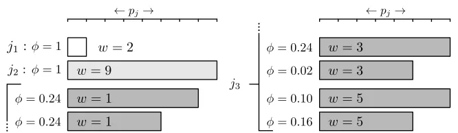
Proof. Consider the following instance with three jobs. Both job 1 and

job 2 have a type space containing only one type, type (w1, p1) = (2,1) and

(w2, p2) = (9,8) respectively. Job 3 has type space (w3, p3)∈ {1,3,5}×{5,7} and the corresponding probabilities for its types are listed below.

φ3(1,5) = 0.24 φ3(1,7) = 0.24 φ3(3,5) = 0.02

φ3(3,7) = 0.24 φ3(5,5) = 0.16 φ3(5,7) = 0.10

Figure 2: Graphical representation of the instance for which the optimal allocation rule does not satisfy the IIA condition.

type of job 3. We will denote these six type profiles by different cases

casea: (w3, p3) = (1,5) caseb: (w3, p3) = (1,7)

casec: (w3, p3) = (3,5) cased: (w3, p3) = (3,7)

casee: (w3, p3) = (5,5) casef : (w3, p3) = (5,7).

For this instance IIA implies that for all six cases, i.e. type profiles, the allocation rule must choose a schedule in which the relative order of job 1

and job 2 is the same16. Therefore the allocation rule must choose schedules

from either{123,132,312}or{213,231,321}for all six cases.

As an example we compute the minimal expected total payments achieved

by allocation rule f, that assigns the following schedules to reported types.

casea→123 case b→123 case c→132

cased→123 case e→132 case f →312

Since we consider a BNIC setting, we take into account individual rationality constraints (2.8) and incentive constraints (2.6). For job 1 and 2 we do not need to take into account incentive constraints as they only have one type. In order to evaluate the individual rationality constraints we need to compute the expected start times for job 1 and 2. These are computed by considering the start time of the job in the schedules assigned to the six cases and account for the probability for each case. For job 1 the minimal expected payment that is enforced by the individual rationality constraint, equals

Eπ₁f(2,1) =w1·ES1(f,2,1)

= 2·(0.24·0 + 0.24·0 + 0.02·0 + 0.24·0 + 0.16·0 + 0.10·7)

= 1.40

16

whereas for job 2 we have

Eπf₂(9,8) =w2·ES2(f,9,8)

= 9·(0.24·1 + 0.24·1 + 0.02·6 + 0.24·1 + 0.16·6 + 0.10·8)

= 23.40.

For job 3 we have to take into account both the incentive and the indi-vidual rationality constrains, both implying a lower bound on the expected payments. Note that although we still refer to them as expected start times, the start times for job 3 are not expected since job 1 and job 2 have only 1 type. Therefore we only have to consider the start time of job 3 in the schedule assigned to the corresponding case. Individual rationality (IRE) for job 3 requires

Eπf₃(1,5), Eπf₃(1,7)≥1·9 = 9

Eπf₃(3,7)≥3·9 = 27

Eπf₃(3,5)≥3·1 = 3

Eπf₃(5,5)≥5·1 = 5

Eπf₃(5,7)≥5·0 = 0.

There are 21 incentive constraints17and therefore it may seem hard to check

if all constraints are fulfilled. However, due to the individual rationality constraints (2.8), the left-hand side of incentive constraints (2.6) is triv-ially greater or equal to zero. Therefore we only need to consider incentive constraints for which the right-hand side is greater than zero. For these con-straints we modify the payments in order to fulfil the incentive concon-straints. This will influence also the right-hand side of the other incentive constraints and therefore we iteratively check all incentive constraints for which the right-hand side is greater than zero and modify the payments until all

in-centive constraints are fulfilled18. In our first iteration we observe that the

17

Remember that we assume that jobs can only overstate their processing time.

18

only incentive constraints that remain are

Eπ₃f(1,5)−1·ES3(f,1,5)≥Eπ3f(3,5)−1·ES3(f,3,5) Eπ₃f(1,5)−1·ES3(f,1,5)≥Eπ₃f(3,7)−1·ES3(f,3,7) Eπ₃f(1,5)−1·ES3(f,1,5)≥Eπ₃f(5,5)−1·ES3(f,5,5) Eπ₃f(3,5)−3·ES3(f,3,5)≥Eπ3f(5,5)−3·ES3(f,5,5) Eπ₃f(1,7)−1·ES3(f,1,7)≥Eπ₃f(3,7)−1·ES3(f,3,7).

By settingEπ₃f(1,5), Eπ₃f(1,7)≥27 andEπf₃(3,5)≥5 these constraints are

fulfilled and in our second iteration we notice that no right-hand side of any incentive constraint is greater than zero. Therefore the minimal payments to job 3 are

Eπf₃(1,5) =Eπf₃(1,7) =Eπ₃f(3,7) = 27

Eπf₃(3,5) =Eπf₃(5,5) = 5

Eπf₃(5,7) = 0.

Now we have computed the minimal expected payments to all jobs, we can

compute the minimal expected total payment achieved by allocation rulef.

EPmin(f) = 1·Eπf₁(2,1) + 1·Eπ₂f(9,8) + X

t3∈T3

φ3(t3)Eπf3(t3)

= 1.40 + 23.40 + 0.24·27 + 0.24·27 + 0.02·5

+ 0.24·27 + 0.16·5 + 0.10·0

= 45.14

In the same way we can compute the minimal expected total payments

achieved by all other 2·36−1 = 1457 allocation rules that are IIA. For this

instance it turns out that allocation rule f is the unique Bayes-Nash

im-plementable allocation rule that achieves minimal expected total payments, while satisfying the IIA condition.

Now consider allocation rule g, that chooses for each case/type profile

the following schedule.

casea→123 case b→123 case c→231

cased→123 case e→132 case f →312

This allocation rule clearly does not satisfy the IIA condition as the relative

the relative order in the schedule chosen for the rest of the cases, although the types of job 1 and job 2 are for all cases identical. Using exact the same

approach as for allocation rule f, we can calculate the payment scheme

corresponding to allocation rule g. For job 1 and 2 again only considering

the individual rationality constraints, the minimal payments to job 1 and job

2 areEπ₁g(2,1) = 1.92 andEπ₂g(9,8) = 22.32. Computing by the individual

rationality constraints for job 3 a lower bound on the expected payments and again iteratively checking the incentive constraints, leads to

Eπ₃g(1,5)≥27 Eπg₃(1,7)≥27 Eπg₃(3,5)≥26 Eπ₃g(3,7)≥27 Eπg₃(5,5)≥5 Eπg₃(5,7)≥0.

For allocation ruleg the minimal expected total payment is

EPmin(g) = 1·Eπg₁(2,1) + 1·Eπ₂g(9,8) + X

t3∈T3

φ3(t3)Eπ3g(t3)

= 1.92 + 22.32 + 0.24·27 + 0.24·27 + 0.02·26

+ 0.24·27 + 0.16·5 + 0.10·0

= 45.00.

This proves the claim.

Now Theorem 1 has been proven, an obvious question is for which spe-cific instances the optimal allocation rule for the 2-dimensional scheduling problem does satisfy the IIA condition. A type of instance we have investi-gated, is one in which jobtypes have a product distribution (see Definition 9). For this type of instance we were not able to find an example for which the optimal allocation rule does not satisfy the IIA condition.

Conjecture 1. For the 2-dimensional scheduling problem, where the types of a job have a product distribution, the optimal allocation rule satisfies the IIA condition.

Despite extensive computational research, we were not able to find an instance contradicting Conjecture 1. Further research will have to verify our conjecture.

5.2 BNIC-DSIC Equivalence

the same solution method as in the previous section, we came to the following result.

Theorem 2. For the 2-dimensional scheduling problem there is in general not a mechanism that is dominant strategy incentive compatible, individu-ally rational and minimizes the expected total payment made to jobs, that achieves the same expected total payments as the optimal mechanism.

Proof. Consider the following instance with two jobs. Job 1 has type space

W1×P1 ={5,7}×{3,7}and job 2 has type spaceW2×P2 ={2,4,7}×{5,6}.

The corresponding probabilities for the jobs’ types are

φ1(5,3) = 0.5 φ1(5,7) = 0.3 φ1(7,3) = 0.1 φ1(7,7) = 0.1

φ2(2,5) = 0.2 φ2(2,6) = 0.0 φ2(4,5) = 0.0 φ2(4,6) = 0.5

φ2(7,5) = 0.3 φ2(7,6) = 0.0.

We will show that for this instance there is no allocation rule that is dom-inant strategies implementable and achieves the same expected total pay-ments as the optimal allocation rule.

The instance has 2 different schedules and as job 1 has four types and job 2 has six types, there are 24 different type profiles. We will denote each

of these type profiles (w1, p1); (w2, p2) by a different case.

casea= (5,3),(2,5) caseb= (5,3),(2,6) case c= (5,3),(4,5)

cased= (5,3),(4,6) casee= (5,3),(7,5) case f = (5,3),(7,6)

caseě = (5,7),(2,5) caseh= (5,7),(2,6) case i= (5,7),(4,5)

casej = (5,7),(4,6) casek= (5,7),(7,5) case l= (5,7),(7,6)

casem= (7,3),(2,5) casen= (7,3),(2,6) case o= (7,3),(4,5)

casep= (7,3),(4,6) caseq = (7,3),(7,5) case r= (7,3),(7,6)

cases= (7,7),(2,5) caset= (7,7),(2,6) case u= (7,7),(4,5)

casev= (7,7),(4,6) casew= (7,7),(7,5) case x= (7,7),(7,6)

Let us first compute the payments made by the optimal mechanism.

In total there are 224 = 16.777.216 allocation rules. For this instance the

unique optimal allocation rule f assigns the following schedules19 to each

case.

casea, b, d,ě, h, m, n, o, p, q, s, t, u, v, w→12 casec, e,f, i, j, k, l, r, x→21

19

Computing the expected start times of job 1, the individual rationality con-straints for this job state

Eπ₁f(5,3)≥5·ES1(f,5,3) = 5·1.5 = 7.5

Eπ₁f(5,7)≥5·ES1(f,5,7) = 5·4.5 = 22.5

Eπ₁f(7,3)≥7·ES1(f,7,3) = 7·0.0 = 0

Eπ₁f(7,7)≥7·ES1(f,7,7) = 7·0.0 = 0.

As in the previous section we iteratively regard the incentive constraints for which the right-hand side exceeds zero. It happens to be that already in the first step all incentive constraints are fulfilled. Therefore, for job 1 the payments are determined only by the individual rationality constraints. For job 2 the individual rationality constraints state

Eπf₂(2,5)≥9.2 Eπf₂(2,6)≥9.2 Eπ₂f(4,5)≥4.0 Eπf₂(4,6)≥10.0 Eπf₂(7,5)≥7.0 Eπ₂f(7,6)≥0.0. The incentive constraints for which the right-hand side exceeds zero are

Eπf₂(2,5)−2·ES2(f,2,5)≥Eπf₂(4,5)−2·ES2(f,4,5) Eπf₂(2,5)−2·ES2(f,2,5)≥Eπf₂(4,6)−2·ES2(f,4,6) Eπf₂(2,5)−2·ES2(f,2,5)≥Eπf2(7,5)−2·ES2(f,7,5) Eπf₂(2,6)−2·ES2(f,2,6)≥Eπf₂(4,6)−2·ES2(f,4,6) Eπf₂(4,5)−4·ES2(f,4,5)≥Eπf₂(7,5)−4·ES2(f,7,5).

From this follows that Eπ₂f(2,5), Eπ₂f(2,6)≥14.2 and Eπ₂f(4,5)≥7.

Re-garding anew the incentive constraints with right-hand side greater than zero, we notice that already in the second iteration, all incentive constraints are fulfilled. Therefore the expected total payment achieved by allocation

rulef is

EPmin(f) = X t1∈T1

φ1(t1)Eπf1(t1) +

X

t2∈T2

φ2(t2)Eπf2(t2)

= 0.5·7.5 + 0.3·22.5 + 0.1·0 + 0.1·0 + 0.2·14.2 + 0.0·14.2 + 0.0·7.0 + 0.5·10.0 + 0.3·7.0 + 0.0·0.0

= 20.44.

payments made to jobs. This happens to be allocation rule f, the same allocation rule that is optimal for the BNIC setting. As we consider a DSIC setting, we take into account individual rationality constraints (2.7) and in-centive constraints (2.5). Apart from the fact that we consider the IR and DSIC constraints, we apply the same method as for the BNIC setting.

De-note by π₁f(α) and π₂f(α) the payment to job 1 and job 2 for case α, under

allocation rule f, respectively. For example, if α = (t1, t2), we denote by

πf₁(α) the payment to job 1, given that it reports type t1 and job 2 reports

type t2. The individual rationality and incentive constraints for job 1 and job 2 imply

π₁f(c)≥25 π₁f(e)≥25 π₁f(f)≥42 πf₁(i)≥25 π₁f(j)≥30 π₁f(k)≥25 π₁f(l)≥42 πf₁(r)≥42 π₁f(x)≥42

π₂f(a)≥12 π₂f(b)≥12 π₂f(d)≥12 πf₂(ě)≥14 π₂f(h)≥14 π₂f(m)≥21 π₂f(n)≥12 πf₂(o)≥21 π₂f(p)≥12 π₂f(q)≥21 π₂f(s)≥49 πf₂(t)≥28 π₂f(u)≥49 π₂f(v)≥28 π₂f(w)≥49

whereas all other payments equal 0. Using this payment scheme we can

compute the expected payment to jobj when it reports typetj, in order to

compare it to the expected payment in the BNIC setting20. We notice that

all expected payments are similar, except for the expected payment to job

2 reporting type (2,5), which occurs in cases a,ě, m, s. Let us denote by

(t1,(2,5)) the case where job 1 reports typet1 and job 2 reports type (2,5),

then for the DSIC setting we have

X

t1∈T1

φ1(t1)·π2f(t1,(2,5)) = 0.5·12 + 0.3·14 + 0.1·21 + 0.1·49 = 17.2

while in the BNIC setting we have Eπf₂(2,5) = 14.2. The raise of this

expected payment by 3, compared to the BNIC case, should be solely re-sponsible for the raise in expected total payments to the jobs in comparison to the BNIC setting. The minimal expected total payment achieved by

al-location rule f for the DSIC setting can be computed by summing over all

cases for all jobs and multiplying by the corresponding probability. Denoting

20

byφ(i) the probability on case, or equivalently, type profile i, we have

Pmin(f) =X j∈J

X

tj∈Tj X

t−j∈T−j

φj(tj)φ−j(t−j)πjf(tj, t−j) = 21.04.

Note that as expected, Pmin(f)−EPmin(f) = 0.2·3 = 0.6, due to the

raise in expected payment to job 2, reporting type (2,5), and the fact that

φ2(2,5) = 0.2.

As for the previous section, there still might be specific instances for which BNIC-DSIC equivalence holds. However, instances where types of jobs have product distributions do not belong to that group.

Theorem 3. For the 2-dimensional scheduling problem, where types of jobs have a product distribution, Bayes-Nash and dominant strategy incentive compatibility is not equivalent.

Proof. Consider the following instance with two jobs. Job 1 has type space

W1×P1 ={3,6} × {2,5} and job 2 has type space W2×P2 ={4,5,9} ×

{1,8}. Note that the probability distribution φj for the type of job j is a

product distribution and therefore we have weight probabilitiesϕj(wj) and

processing time probabilitiesψj(pj).

ϕ1(3) = 0.4 ϕ1(6) = 0.6 ψ1(2) = 0.3 ψ1(5) = 0.7

ϕ2(4) = 0.4 ϕ2(5) = 0.2 ϕ2(9) = 0.4 ψ2(1) = 0.5 ψ2(8) = 0.5.

Note that from these probabilities follow the corresponding probabilities for types of jobs. We will show that for this instance there is no DSIC mecha-nism that is individually rational and achieves the same minimal expected total payments as the optimal mechanism.

Computing the minimal expected total payments for both the BNIC and DSIC setting, is similar to the previous example and therefore we omit most of the steps. The instance has 2 different schedules and 24 different type profiles, which we all denote by a different case.

case a= (3,2),(4,1) caseb= (3,2),(4,8) case c= (3,2),(5,1)

case d= (3,2),(5,8) casee= (3,2),(9,1) case f = (3,2),(9,8)

case ě= (3,5),(4,1) caseh= (3,5),(4,8) case i= (3,5),(5,1)

case j= (3,5),(5,8) casek= (3,5),(9,1) case l= (3,5),(9,8)

case m= (6,2),(4,1) casen= (6,2),(4,8) case o= (6,2),(5,1)

case p= (6,2),(5,8) caseq = (6,2),(9,1) case r= (6,2),(9,8)

case s= (6,5),(4,1) caset= (6,5),(4,8) case u= (6,5),(5,1)

For each of these cases we must compute the (expected) payments made to the jobs. Let us first compute the expected total payments made by the

optimal mechanism. In total there are 224_{= 16.777.216 allocation rules. It}

turns out that for this instance there are two optimal allocation rules. We

will consider optimal allocation rule f, that assigns the following schedules

to each case.

case b, d, h, m, n, o, p, t, v→12

case a, c, e,f,ě, i, j, k, l, q, r, s, u, w, x→21

Considering individual rationality constraints (2.8) and incentive constraints (2.6) for both job 1 and job 2, we obtain lower bounds on the expected payments.

Eπ₁f(3,2)≥12.60 Eπ₁f(3,5)≥15.00 Eπ₁f(6,2)≥10.80 Eπ₁f(3,2)≥12.60

Eπ₂f(4,1)≥4.14 Eπ₂f(4,8)≥19.10 Eπ₂f(5,1)≥4.14 Eπ₂f(5,8)≥13.50 Eπ₂f(9,1)≥0.90 Eπ₂f(9,8)≥0.00 This leaves us to compute the expected total payment achieved by allocation

rule f, which is

EPmin(f) = X t1∈T1

φ1(t1)Eπf₁(t1) +

X

t2∈T2

φ2(t2)Eπf₂(t2)

= 0.12·12.60 + 0.28·15.00 + 0.18·10.80 + 0.42·12.60 + 0.20·4.14 + 0.20·19.10 + 0.10·4.14 + 0.10·13.50 + 0.20·0.90 + 0.20·0.00

= 19.54.

Now we compute the payments achieved by the allocation rule that is dominant strategy implementable, individually rational and minimizes the

expected total payments made to jobs. This is allocation ruleg, that assigns

the following schedules to each case.

case b, d, h, m, n, o, p, r, t, v→12

case a, c, e,f,ě, i, j, k, l, q, s, u, w, x→21