using Constant Shape Weibull Mixture ROC Curve
Sudesh Pundir
Department of Statistics, Pondicherry University, Puducherry, India [email protected]
Azharuddin
Department of Statistics, Pondicherry University, Puducherry, India [email protected]
Abstract
Receiver Operating Characteristic (ROC) Curve is a widely used classification technique in Medical Diagnosis which classifies the healthy and diseased individuals on the basis of optimal cut off value of the biomarker. In this article, we have proposed Constant Shape Weibull Mixture ROC (CSWMROC) model. The properties of CSWMROC Curve are discussed and expressions for AUC, its variance and confidence interval are derived. The estimates of AUC of CSWMROC curve are obtained using Method of Moments (MOM). Numerical example is considered to support the proposed theory.
Keywords: CSWMROC Curve, AUC, Optimal cut-off value, Method of Moments, Monte Carlo simulation.
1. Introduction
Weibull Mixture distribution is very useful in medical diagnosis because it attains many shapes for different values of shape and scale parameters which helps in modeling different types of data. Here, we keep constant shape parameter to obtain the proper CSWMROC Curve so that it never crosses the chance diagonal otherwise it will become worthless.
Only a limited literature is available on the mixture of distributions. Some books on finite mixture distributions are written by Everitt and Hand [1981], Titterington et al. [1985] and McLachlan and Peel [2000]. Some authors like Newcomb [1886] studied the finite mixture distributions for outlier and Pearson [1894] estimated the parameters of the two component normal-mixture distribution by using the method of moments.
mean error and time completion of the algorithm using different method of estimation by simulation studies. Pundir and Amala [2014] proposed and discussed the characteristics of the constant shape weibull ROC Curve.
ROC Curve is a graph between False positive rate (x(t)) and True positive rate (y(t)) for cut off value t. Till date, there are many authors like Green and Swets in [1966], Egan [1975], Zhou et al. [2002] and Krzanowski and Hand [2002] who discussed the ROC Curve for univariate distributions in case of continuous data. They gave the idea on theory of estimation on ROC Curve, AUC of ROC Curve and also used Statistical Inference on ROC Curve.
In practice, medical data is heterogeneous or it may consist of sub populations. Generally, we ignore this fact and apply the existing ROC models without checking for the heterogeneity which gives us the misleading results. Hence, there is a need to introduce mixture ROC models which will give exact accuracy of the diagnostic test with less standard error.
Only few authors discussed the mixture ROC Curve. The first article on the mixture ROC Curve is given by Dass and Kim [2011] where they discussed the Multivariate Bi-normal Mixture ROC Curve. Gonen [2013] also studied the ROC Curve and AUC using Bi-normal mixture distribution. It was found that if the heterogeneity is found in the data then Bi-normal mixture ROC Curve gives better smoothness as compare to bi-normal ROC Curve. Pundir and Azharuddin [2014] studied the Exponential Mixture ROC Curve and compared the estimates of AUC of Exponential Mixture ROC Curve using Method of Moments and MLE. Pundir and Azharuddin [2016] studied the Normal Mixture ROC Curve along with its properties and found the maximum likelihood estimates of parameters of AUC and confidence interval of AUC of Normal Mixture ROC Curve. A mixture distribution can be applied if a population contains two or more sub-populations or in the presence of heterogeneity. A random variable X is said to follow a mixture distribution if it has the probability density function as
/
, 0, 1,2,..., 11 1
k
i i k
i
i i i
if x p i k and p
p x
f
(1.1)
wherepi is the weight of the ith component of mixture distribution.
A class N of mixture is said to be identifiable if and only if for all f
x N and the equality of two representations
jn
j
j j i
n
i i
i
f
x
p
f
x
p
;
ˆ
;
ˆ
'
1
1
(1.2)holds where, n=n’ and for all i there exit some j such that pi pˆjand i ˆj. A random variable X is said to follow the two component weibull mixture distribution with probability density function
exp
1
exp , 0 , 0 , 0 , 1,2. 21
2 2
1 1
1 1
2 2
1
1
i x
x x
p x
x p x
f i i
(1.3)
The cumulative distribution function of the two component weibull mixture distribution is given as
1 exp
1
1 exp 0 , 0 , 0 , 1,2.2 1
2 1
p x p x x i
x
F i i
(1.4) where
iand
i are the shape and scale parameters of the weibull mixture distribution. In this paper, the shape parameter 1 2 is constantThe paper is organized as follows. In section 2, we have studied the CSWMROC model and its properties. The AUC and optimal cut-off value of biomarker using CSWMROC model are also derived. The moment estimates of AUC of CSWMROC Curve are also obtained in section 3. In section 4, the variance of AUC of CSWMROC model and confidence Interval (CI) are derived using delta method. In section 5, AUC, variance of AUC, Standard Error (SE) of AUC, Mean Square Error (MSE) of AUC, confidence interval and testing of AUC are done by using simulation studies. In the last section, conclusion is given.
2. Constant Shape Weibull Mixture ROC model
Let X be a random variable from healthy controls which follows Constant Shape Weibull Mixture Distribution with parameters ,10and 20 and Y be another random variable
from disease cases which follows Constant shape Weibull Mixture Distribution with parameters ,11and 21. The CSWMROC model is defined as
(2.1) where,
Assumptions:
(1) The mean of disease cases should be greater than the mean of healthy cases for CSWMROC curve.
1
21, 0 1;0 ;0 ; 0,1; 1,2.20 11
10
p xt p xt p t i j
t
y ij
exp
1
exp .20 10
t p
t p
(2) The Shape parameter ( ) should be fixed to obtain the proper CSWMROC curve.
(3) 1110, 2120 , 2010 and 2111.
Properties:
(a) The CSWMROC curve remains unaltered if the test scores undergo a strictly increasing transformation.
(b) CSWMROC curve is monotonically increasing.
Proof: A function is said to be monotonically increasing function if the first derivative of the function is greater than zero. From (2.1), we have
10 20 11 21 1 1 10 20 0 1 11 211 0, 0, i 0, i 0, 1, 2.
dy t
p y t p x t p i
dx t
(2.2)
(c) CSWMROC Curve is a Concave.
Proof: A function is said to be concave if its second derivative is less than zero. From (2.2), we have
1
1
1
0, 0, 0 0, 1 0, 1,2.2 21 20 21 20 2 11 10 11 10 2 2 21 20 11 10 i p t x p t y p t dx t y d i i (2.3)
(d) CSWMROC Curve is TPR asymmetric.
Proof: Let f(x) be comparison distribution and g(x) be reference distribution, then KL(f, g) and KL(g, f) are given as
21 21 11 11 20 10 10 20 21 11 21 11 11 21 20 10 exp 1 1 exp 1 exp 1 exp ln ln ln exp 1 exp ln ln ln , t p t p t p t p t p t p g f KL (2.4)
1 1 exp . exp 1 exp 1 exp ln ln ln exp 1 exp ln ln ln , 20 20 10 10 21 11 11 21 20 10 20 10 10 20 21 11 t p t p t p t p t p t p g f KL (2.5)
From (2.4) and (2.5), we can see that KL(g, f) > KL(f, g) i.e. the CSWMROC Curve is TPR asymmetric.
(e) The slope of the CSWMROC Curve at the cut off value t is given as
(2.6)
1
exp .The AUC of CSWMROC Curve is defined as
(2.7)
Optimal cut-off value
In medical diagnosis, the optimal cut-off value (t) tells us about the patient’s situation whether his status of disease. The optimal cut-off value is defined by the Fluss et al. (2005) in the Youden index which is obtained by taking the maximum difference between the CDF of healthy and disease cases. The optimal threshold value or cut-off value of biomarker using CSWMROC curve is obtained as
(2.8)
3. Estimates of parameters of AUC of CSWMROC Curve using Method of Moments
It is very old and easy method for estimating the parameters. The rth sample moment of a mixture distribution is defined as
(3.1) where, f1
x and f2
x are the densities of two sub-populations of mixture distribution. The rth sample moment of Constant Shape Weibull Mixture distribution is obtained as
1
exp .exp
2 0
1 2
1 0
1 1
'
dx x x
p dx
x x
p
mr r r
(3.2)
The shape parameter is constant for both sub populations and 1 and 2are the scale parameters of Weibull Mixture distribution. On putting r=1, 2, 3, 4 in (3.2), we get
1
1 1
1
1 201/
/ 1 10 '
1 p p
m (3.3)
2
1 1
2
1 202/
/ 2 10 '
2 p p
m (3.4)
3
1 1
3
1 203/
/ 3 10 '
3 p p
m (3.5)
4
1 1
4 1
.'4 p 104/ p 204/
m (3.6)
On solving (3.3)-(3.6), one can obtain pˆ,ˆ, ˆ1,and ˆ2 by using the Newton Raphson method in MATHEMATICA software.
1
ln .ln
20 21
20 21
20 21
10 11
10 11
10 11
max
max
t t
p t
p
1
( 1) (1 )( 2).21 20
21 11
10 11
AUC p AUC
p p
p
AUC
x r x
r
r p x f x dx p x f x dx
m 1 2
'
4. Variance of AUC of CSWMROC Curve using delta method
The approximate variance of AUC of CSWMROC Curve by Delta method gives the approximate variance as
ˆ
ˆ 1
ˆ 2
V AUC pV AUC 1 p V AUC (4.1)
where
11 10
11
1
AUC and .
21 20
21
2
AUC (4.2)
Using delta method, we have
20 21 20 2 21 2 20 2 20 2 21 2 21 2 2 10 11 10 1 11 1 10 2 10 1 11 2 11 1 1 ˆ , ˆ cov 2 ˆ ˆ ˆ ˆ , ˆ cov 2 ˆ ˆ ˆ AUC AUC V AUC V AUC C U A V AUC AUC V AUC V AUC C U A V (4.3)On substituting (4.3) in (4.1), we get
1
ˆ
ˆ 2 cov
ˆ , ˆ
.ˆ , ˆ cov 2 ˆ ˆ ˆ 20 21 20 2 21 2 20 2 20 2 21 2 21 2 10 11 10 1 11 1 10 2 10 1 11 2 11 1 AUC AUC V AUC V AUC p AUC AUC V AUC V AUC p C U A V (4.4)
Differentiating (4.2) with respect to 11,10,21 and 20, we get
220 21 21 20 2 2 20 21 20 21 2 2 10 11 11 10 1 2 10 11 10 11 1 , , ,
AUC AUC AUC AUC
To determine the variance of ˆ11,ˆ10,ˆ21 and ˆ20, we use the Fisher information matrix. The likelihood function is given as
. 11 10 1 11 1 10
n j m i y g x f LThe Fisher information matrix is given as
where,
10 11
1 , ,
10 ' 2 10 10 31 13 32 23 11 , 2 11 11 21 12 2 10 10 33 2 11 11 22 2 10 10 2 11 11 ' 2 10 10 11 11 , 2 11 10 11 ln 0 , ln , , ln ln ln ln 2 1 m a a a a n a a m a n a m n m n n m a (4.6) and
' ! n n k 1 1 1 n 1 n k , : Euler-Mascheroni constant approximately equal to 0.5772
20 10,m
m : sample sizes of healthy controls
21 11,n
n : sample sizes of disease cases.
On substituting(4.6) in (4.5), the inverse Fisher Information matrix is given as
22 33 21 33 22 31
1 2
1 2 2 12 33 11 33 13 12 31
11 22 33 12 33 22 13 2
22 13 21 13 11 22 12
a a a a a a
1
I a a a a a a a
a a a a a a a
a a a a a a a
10 11 10 10 10 11 11 11 10 11 ˆ ˆ , ˆ ˆ , ˆ ˆ , ˆ ˆ ˆ , ˆ ˆ , ˆ ˆ , ˆ ˆ V COV COV COV V COV COV COV V (4.7) where
2 ' 2 " 2 11 10 11 , 2 10 ' 2 11 10 10 11 2 ' 2 " 2 11 10 11 ' 2 11 11 2 ' 2 " 2 10 11 10 11 2 ' 2 2 11 2 10 11 10 ' 2 10 10 11 " 2 10 11 11 2 10 10 2 ' 2 " 2 10 11 10 11 2 ' 2 2 10 2 11 11 10 ' 2 11 10 11 " 2 10 11 11 2 11 11 11 10 10 ' 2 10 10 , 2 " 2 11 10 2 1 ln ln ˆ , ˆ cov , 1 ln ˆ , ˆ cov , 1 log log 2 1 ˆ , 1 log log 2 1 ˆ , ln ˆ , ˆ cov , 1 ˆ ' 2 n m n m m n m n n n m m n m n n V m n m n m n m m n m n n V n m n m V (4.8)
''
' 2
On putting (4.8) in (4.3), V
AUˆC1 is given as
. 1 ln ˆ 2 ' 2 " 2 10 11 2 11 10 10 11 10 11 4 10 11 2 10 2 11 1 m n m n m n C U A V (4.9)Similarly, the V
AUˆC2
is given as
1
.ln ˆ 2 ' 2 " 2 20 21 2 21 20 20 21 20 21 4 20 21 2 20 2 21 2 m n m n m n C U A V (4.10)
On substituting (4.9) and (4.10) in (4.1), we get
(4.11)
Using V(AUC), one can easily find confidence interval, MSE and test of significance for AUC.
(i) The 100(1-α)% confidence interval of AUC is given as
ˆ
2 Z C U A SE AUC (4.12) where α is the level of significance and
2
Z is the critical value of the confidence interval and SE is the standard error.
(ii) The Mean Square Error (MSE) is used to identify the quality of an estimator. It is defined as
ˆ
ˆ
ˆ
2C U A Bias C U A Variance C U A
MSE (4.13)
1
.where
(iii) Consider the problem of testing of AUC of CSWMROC Curve as 0
0:AUC AUC
H vs. H1:AUCAUC0.
The test statistic is given as
~
0,1 ˆˆ
N C
U A V
AUC C
U A N
Z
(4.14)
where N = m + n, m is the sample size of healthy controls and n is the sample size of disease cases.
5. Simulation Studies
The random numbers are generated from Weibull mixture distribution with fixed values of shape parameter and scale parameters of healthy controls and disease cases for the sample sizes N=10, 20, 30, 100, 200 and 300. The sample sizes are equal for healthy controls and disease cases. The value of weight of healthy controls and disease case are also taken as equal i.e., p=0.7. The values of shape parameter is same for healthy controls and disease cases 102011212. The values of scale parameters of
healthy controls and disease cases are 10 1, 20 2 and 1110, 219.
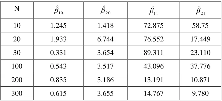
Table 5.1: Estimates of parameters of AUC of CSWMROC Curve by MOM for different sample sizes
N
10
ˆ
ˆ20 ˆ11 ˆ21
10 1.245 1.418 72.875 58.75
20 1.933 6.744 76.552 17.449
30 0.331 3.654 89.311 23.110
100 0.543 3.517 43.096 37.776
200 0.835 3.186 13.191 10.871
300 0.615 3.655 14.767 9.780
From above table, it is observed that with the increase in sample size, the estimates of CSWMROC model become closer to the parameters. Using the estimators in Table 5.1, one can see AUˆC, V
AUˆC, SE AUˆC , confidence interval and Z-values to test A in Table 5.2.
AUˆC E AUˆC AUC.Table 5.2: AUˆC, V
AUˆC, SE AUˆC ,MSE
AUˆC , 95% Confidence Interval (CI) ofC U
A ˆ and Z-values
N AUˆC V
AUˆ C SE
AUˆC MSE
AUˆ C CI
AUˆ C Z-values 10 0.981 0.0002 0.0152 0.0101 [0.951, 1.01] 31.939 20 0.899 0.0015 0.0387 0.0018 [0.823, 0.975] 3.102 30 0.956 0.0004 0.0206 0.0059 [0.916, 0.996] 29.434 100 0.965 0.0000 0.0087 0.0071 [0.948, 0.982] 120.208 200 0.890 0.0001 0.0126 0.0002 [0.865, 0.915] 20.00 300 0.890 0.0001 0.0103 0.0001 [0.870, 0.910] 24.494 It is observed from Table 5.2 that AUˆC become closer to the true value of AUC as the sample size increases but V AUC
ˆ , SE
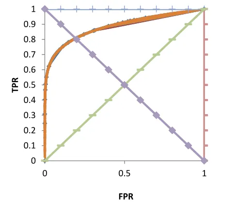
AUˆC and MSE(AUC) decreases with increase in the sample size because the variance of AUC and standard error of AUC depends on sample sizes. From Z values, one can see that all AUˆCvalues are greater than 0.88, so we reject the null hypothesis and concludes that AUC is not equal to 0.88.Fig. 5.1 shows the CSWMROC curves for different sample sizes and fixed values of parameters mentioned above.
Fig. 5.1 CSWMROC Curve with fixed parameters and different sample sizes.
0 0.1 0.2 0.3 0.4 0.5 0.6 0.7 0.8 0.9 1
0 0.5 1
TPR
6. Conclusion
In this paper, we have proposed CSWMROC model and found that CSWMROC curve is monotonically increasing, concave in nature and TPR asymmetric. The Area under the CSWMROC Curve, its variance and the optimal cut-off value of biomarker using CSWMROC Curve are also derived. The estimates of parameters of AUC are obtained by MOM. The variance of AUC of ROC Curve is also derived. The MSE of AUC, confidence interval of AUC and test for AUC are also discussed. From simulation studies, it is concluded that the estimates of parameters of AUC of CSWMROC Curve using MOM become approximately closer to the population parameters for large sample size. It is concluded that when heterogeneity is found in the data and Weibull mixture distribution fits well to the data then one should use Weibull mixture ROC model instead of Bi-Weibull ROC model.
References
1. Arfa M. and Aslam M. (2008). “A comparative study to estimate the parameters of mixed-weibull distribution”, Pak.J.Stat.Oper.Res., 4(1), 1-8.
2. Atienza N., Garcia-Heras J., and Munoz Pichardo J. m. (2006). “A new condition for Identifiability of finite mixture distributions”. Metrika (2006) 63:215-221, Doi 10.1007/s00184-005-0013-z.
3. Bucar T., Nagode M., and Fajdiga M. (2003). “Reliability approximation using finite Weibull mixture distributions”, Reliability Engineering and System Safety, 84, 241–251.
4. Dass S.C. and Kim S.W. (2011). “A Semi-parameteric Approach to Estimation of ROC Curves for Multivariate Binormal Mixtures”, www.stt.msu.edu/Links/Research_Memoranda/RM/RM_683.pdf.
5. Dewan I. and Nandi S. (2009). “An em algorithm for estimating the parameters of bivariate weibull distribution under random censoring”,
www.isid.ac.in/~statmath/eprints.
6. Dwidayati N. et al (2013). “Estimation of the Parameters of a Mixture Weibull Model for Analyze Cure Rate”, Applied Mathematical Sciences, 7(116), 5767 – 5778.
7. Egan J.P. (1975). “Signal Detection Theory and ROC Analysis”, Academic Press, New York.
8. Erisoglu U. and Erisoglu M. (2014). “L-Moments estimates for mixture of weibull distributions”, Journal of data science 12, 69-85.
9. Everitt B. and Hand D.J. (1981). “Finite Mixture Distributions”, Chapman and Hall, New York.
10. Fluss, R., Faraggi, D. and Reiser, B. (2005). “Estimation of the Youden Index and its associated cutoff point”, Biometrical Journal, 47(4), 458-472.
12. Green D.M. and Swets J.A. (1966). “Signal Detection Theory and Psychophysics”, Wiley, New York.
13. Kao J.H.K. (1959). “A graphical estimation of mixed weibull parameters in life-testing of electron tubes”, Technometrics 1, 389-407.
14. Krzanowski W.J. and Hand D.J. (2002). “ROC curves for continuous data, Monographs on Statistics and Applied Probability”, CRC Press, Taylor and Francis Group, New York.
15. McLachlan G. and Peel D. (2000). “Finite Mixture Models”, John Wiley, New York.
16. Newcomb S. (1886). “A generalized theory of the combination of observations so as to obtain the best result”, Amer. J. Math, 8, 343-346.
17. Pearson K. (1894). “Contribution to the mathematical theory of evolution”, Phil. Trans. Roy. Soc. A, 185, 71-110.
18. Pundir S. and Amala R. (2014). Evaluation of area under the Constant Shape Bi-Weibull ROC Curve, Journal of Modern Applied Statistical Methods, 13(1), 305-328.
19. Pundir S. and Azharuddin (2014). “A Study of Exponential Mixture ROC Model, 3rd International Conference on Innovative Approach in Applied Physical, Mathematical/Statistical, Chemical Sciences and Emerging Energy Technology for sustainable Development”, 18-26.
20. Pundir S. and Azharuddin (2016). “Detection of AUC and Confidence Interval using Normal Mixture ROC Curve”, IOSR Journal of Mathematics (IOSR-JM), e-ISSN: 2278-5728, p-e-ISSN: 2319-765X. 12(2), 77-86.
21. Teicher, H. (1961). “Identifiability of Mixtures”. The Annals of Mathematical Statistics 32, 244-248.
22. Teicher, H. (1963). “Identifiability of finite Mixtures”, The Annals of Mathematical Statistics 34, 1265-1269.
23. Titterington D.M. et.al (1985). “Statistical Analysis of Finite Mixture Distributions”, John Wiley and Sons Ltd.
24. Yakowitz, S.J. and Spragins, J.D. (1968). “On the Identifiability of Finite Mixtures”, The Annals of Mathematical Statistics, 39, 209-214.
Programs
(a) R-Command
The random numbers are generated by using the following command y<-p*runif(n)+(1-p)*runif(n)
x<-p*((log((1-y)^(-b1)))^(1/a))+(1-p)*((log((1-y)^(-b2)))^(1/a))
n: sample size, a: shape parameter, b1: scale parameter of 1st sub-population, b2: scale parameter of 2nd sub-population.
(b) MATHEMATICA Command
The moment estimators of AUC of CSWMROC Curve are obtained by using the following command
FindRoot[{p*b1^(1/\[Alpha])*Gamma[1 + 1/\[Alpha]] + (1 - p)*b2^( 1/\[Alpha])*Gamma[1 + 1/\[Alpha]] == m1,
p*b1^(2/\[Alpha])*Gamma[1 + 2/\[Alpha]] + (1 - p)*b2^( 2/\[Alpha])*Gamma[1 + 2/\[Alpha]] == m2,
p*b1^(3/\[Alpha])*Gamma[1 + 3/\[Alpha]] + (1 - p)*b2^( 3/\[Alpha])*Gamma[1 + 3/\[Alpha]] == m3,
p*b10^(4/\[Alpha])*Gamma[1 + 4/\[Alpha]] + (1 - p)*b2^( 4/\[Alpha])*Gamma[1 + 4/\[Alpha]] == m4}, {p,p0 }, {\[Alpha], [Alpha0]}, {b1, b10}, {b2, b20}]
(c) Euler-Mascheroni Constant
The first order differentiation of is given asn
n where
n called the digammafunction. The value of n' at n is equal to 1-', where is Euler-Mascheroni constant and its approximate value is 0.5772. The second order differentiation at n is define as
0
2 1
''
logx dx e
xn x
n has the value
.6 1
1
2 2
The general mth derivative of n is obtained by
log
.0 1