www.earth-surf-dynam.net/4/359/2016/ doi:10.5194/esurf-4-359-2016
© Author(s) 2016. CC Attribution 3.0 License.
Image-based surface reconstruction in geomorphometry
– merits, limits and developments
Anette Eltner1, Andreas Kaiser2, Carlos Castillo3, Gilles Rock4, Fabian Neugirg5, and Antonio Abellán6
1Institute of Photogrammetry and Remote Sensing, Technische Universität Dresden, Dresden, Germany
2Soil and Water Conservation Unit, Technical University Freiberg, Freiberg, Germany
3Dept. of Rural Engineering, University of Córdoba, Córdoba, Spain
4Dept. of Environmental Remote Sensing and Geomatics, University of Trier, Trier, Germany
5Dept. of Physical Geography, Catholic University Eichstätt-Ingolstadt, Eichstätt, Germany
6Risk Analysis Group, Institute of Earth Sciences, University of Lausanne, Lausanne, Switzerland
Correspondence to: Anette Eltner ([email protected])
Received: 1 December 2015 – Published in Earth Surf. Dynam. Discuss.: 15 December 2015 Revised: 28 April 2016 – Accepted: 9 May 2016 – Published: 19 May 2016
Abstract. Photogrammetry and geosciences have been closely linked since the late 19th century due to the
acquisition of high-quality 3-D data sets of the environment, but it has so far been restricted to a limited range of remote sensing specialists because of the considerable cost of metric systems for the acquisition and treatment of airborne imagery. Today, a wide range of commercial and open-source software tools enable the generation of 3-D and 4-D models of complex geomorphological features by geoscientists and other non-experts users. In addition, very recent rapid developments in unmanned aerial vehicle (UAV) technology allow for the flexible generation of high-quality aerial surveying and ortho-photography at a relatively low cost.
The increasing computing capabilities during the last decade, together with the development of high-performance digital sensors and the important software innovations developed by computer-based vision and visual perception research fields, have extended the rigorous processing of stereoscopic image data to a 3-D point cloud generation from a series of non-calibrated images. Structure-from-motion (SfM) workflows are based upon algorithms for efficient and automatic orientation of large image sets without further data acqui-sition information, examples including robust feature detectors like the scale-invariant feature transform for 2-D imagery. Nevertheless, the importance of carrying out well-established fieldwork strategies, using proper camera settings, ground control points and ground truth for understanding the different sources of errors, still needs to be adapted in the common scientific practice.
1 Introduction
Early works on projective geometries date back to more than five centuries, when scientists derived coordinates of points from several images and investigated the geometry of per-spectives (Doyle, 1964). Projective geometry represents the basis for the developments in photogrammetry in the late 19th century, when Aimé Laussedat experimented with ter-restrial imagery as well as kites and balloons for obtaining imagery for topographic mapping (Laussedat, 1899). Pho-togrammetry has rapidly advanced to be an essential tool in geosciences during the last two decades and has lately been gaining momentum driven by digital sensors leading to flexible, fast and facile generation of images. Simulta-neously, growing computing capacities and rapid develop-ments in computer vision led to the method of structure from motion (SfM), which opened the way for low-cost, high-resolution topography. Thus, the community using image-based 3-D reconstruction experienced a considerable growth, not only in the quality and detail of the achieved results but also in the number of potential users from diverse geoscien-tific disciplines.
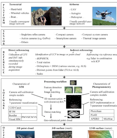
SfM photogrammetry can be performed with images ac-quired by consumer-grade digital cameras and is thus very flexible in its implementation. Its ease of use in regard to data acquisition and processing makes it further interesting to non-experts (Fig. 1). The diversity of possible applica-tions led to a variety of terms used to describe SfM pho-togrammetry either from a photogrammetric or a computer vision standpoint. Thus, to avoid ambiguous terminology, a short list of definitions in regard to the reviewed method is given in Table 1. In this review a series of studies that utilise the algorithmic advance of high automation in SfM are con-sidered – i.e. no initial estimates of the image network ge-ometry or user interactions to generate initial estimates are needed. Furthermore, data processing can be performed al-most fully automatically. However, some parameter settings typical for photogrammetric tools (e.g. camera calibration values) can be applied to optimise both accuracy and preci-sion, and ground control point (GCP) or scale identification is still necessary.
SfM photogrammetry can be applied to a vast range of temporal scales (reaching from sub-second to decades) as well as spatial scales (reaching from sub-millimetre to kilo-metres) and resolutions up to an unprecedented level of de-tail, allowing for new insights into earth surface processes, i.e. 4-D (three spatial dimensions and one temporal di-mension) reconstruction of environmental dynamics. For in-stance, the concept of sediment connectivity (Bracken et al., 2015) can be approached from a new perspective through varying spatio-temporal scales. Thereby, the magnitude and frequency of events and their interaction can also be eval-uated. Furthermore, the versatility of SfM photogrammetry utilising images captured from aerial or terrestrial perspec-tives has the advantage of being applicable in remote areas
with limited access and in fragile, fast-changing environ-ments.
After the suitability of SfM has been noticed for geoscien-tific applications (James and Robson, 2012; Westoby et al., 2012; Fonstad et al., 2013) the number of studies utilising SfM photogrammetry for geomorphometric investigations (thereby referring to the “science of topographic quantifica-tion” based on Pike et al., 2008) has increased significantly. However, the method needs a sophisticated study design and some experience in image acquisition to prevent predictable errors and to ensure good quality of the reconstructed scene. Smith et al. (2015) and Micheletti et al. (2015) recommend a setup for efficient data acquisition.
A total of 65 publications are reviewed in this study. They are chosen according to the respective field of research and methodology. Only those studies that make use of the ben-efits of automatic image-matching algorithms, and thus ap-ply the various SfM tools, are included. Studies that lack full automation are excluded, i.e. some traditional photogram-metric software. Topic-wise, a line is drawn in regard to the term geosciences. The largest fraction of the reviewed articles tackles questions arising in geomorphological con-texts. To account for the versatility of SfM photogramme-try, a few studies deal with plant growth on different scales (moss, crops, forest) or investigate rather exotic topics such as stalagmites or reef morphology.
This review aims to highlight the development of SfM photogrammetry as a valuable tool for geoscientists:
1. The method of SfM photogrammetry is briefly sum-marised, and algorithmic differences due to their emer-gence from computer vision as well as photogrammetry are clarified (Sect. 2).
2. Open-source tools regarding SfM photogrammetry are introduced as well as beneficial tools for data post-processing (Sect. 2).
3. Different fields of applications where SfM photogram-metry led to new perceptions in geomorphophotogram-metry are displayed (Sect. 3).
4. The performance of the reviewed method is evaluated (Sect. 4).
5. Frontiers and significance of SfM photogrammetry are discussed (Sect. 5).
2 SfM photogrammetry: method outline
2.1 Basic concept
Figure 1.Schematic illustration of the versatility of SfM photogrammetry.
of (digital) photogrammetry. Software and hardware devel-opments as well as the increase in computing power in the 1990s and early 2000s made aerial photogrammetric process-ing of large image data sets accessible to a wider community (e.g. Chandler, 1999).
Camera orientations and positions, which are usually un-known during image acquisition, have to be reconstructed to model a 3-D scene. For that purpose, photogrammetry has developed bundle adjustment (BA) techniques, which allow for simultaneous determination of camera orientation and po-sition parameters as well as 3-D object point coordinates for a large number of images (e.g. Triggs et al., 2000). BA
needs image coordinates of many tie points as input data. If the BA is extended by a simultaneous calibration option, even the intrinsic camera parameters can be determined in addition to the extrinsic parameters. Furthermore, a series of ground control points can be used as input into BA for geo-referencing the image block (e.g. Luhmann et al., 2014; Kraus, 2007; Mikhail et al., 2001).
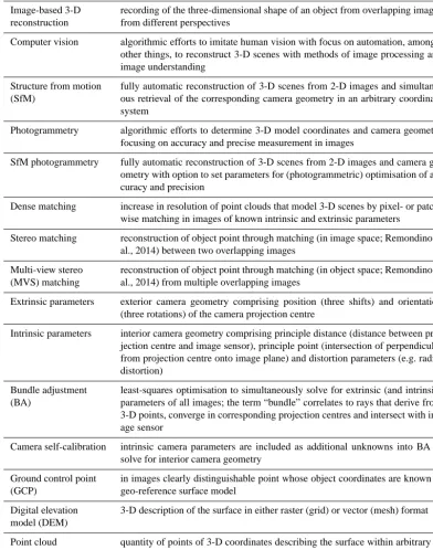
Table 1.Nomenclature and brief definitions of image-based 3-D reconstruction-related terms.
Image-based 3-D reconstruction
recording of the three-dimensional shape of an object from overlapping images from different perspectives
Computer vision algorithmic efforts to imitate human vision with focus on automation, amongst
other things, to reconstruct 3-D scenes with methods of image processing and image understanding
Structure from motion (SfM)
fully automatic reconstruction of 3-D scenes from 2-D images and simultane-ous retrieval of the corresponding camera geometry in an arbitrary coordinate system
Photogrammetry algorithmic efforts to determine 3-D model coordinates and camera geometry
focusing on accuracy and precise measurement in images
SfM photogrammetry fully automatic reconstruction of 3-D scenes from 2-D images and camera
ge-ometry with option to set parameters for (photogrammetric) optimisation of ac-curacy and precision
Dense matching increase in resolution of point clouds that model 3-D scenes by pixel- or patch-wise matching in images of known intrinsic and extrinsic parameters
Stereo matching reconstruction of object point through matching (in image space; Remondino et
al., 2014) between two overlapping images
Multi-view stereo (MVS) matching
reconstruction of object point through matching (in object space; Remondino et al., 2014) from multiple overlapping images
Extrinsic parameters exterior camera geometry comprising position (three shifts) and orientation (three rotations) of the camera projection centre
Intrinsic parameters interior camera geometry comprising principle distance (distance between pro-jection centre and image sensor), principle point (intersection of perpendicular from projection centre onto image plane) and distortion parameters (e.g. radial distortion)
Bundle adjustment (BA)
least-squares optimisation to simultaneously solve for extrinsic (and intrinsic) parameters of all images; the term “bundle” correlates to rays that derive from 3-D points, converge in corresponding projection centres and intersect with im-age sensor
Camera self-calibration intrinsic camera parameters are included as additional unknowns into BA to solve for interior camera geometry
Ground control point (GCP)
in images clearly distinguishable point whose object coordinates are known to geo-reference surface model
Digital elevation model (DEM)
3-D description of the surface in either raster (grid) or vector (mesh) format
Point cloud quantity of points of 3-D coordinates describing the surface within arbitrary or
geo-referenced coordinate system; additional information such as normals or colours possible
technique (Ullman, 1979) allowing for processing of large data sets and the use of a combination of multiple non-metric cameras.
The typical workflow of SfM photogrammetry (e.g. Snavely et al., 2008) comprises the following steps:
1. identification and matching of homologous image points in overlapping photos (image matching; e.g. Lowe, 1999);
2. reconstruction of the geometric image acquisition con-figuration and of the corresponding 3-D coordinates of matched image points (sparse point cloud) with iterative BA;
4. scaling or geo-referencing, which is also performable within step 2.
Smith et al. (2015) give a detailed description of the work-flow of SfM photogrammetry, especially regarding step 1 and step 2.
In contrast to classical photogrammetry software tools, SfM allows for reliable processing of a large number of im-ages in rather irregular image acquisition schemes (Snavely et al., 2008) with a much higher degree of process automa-tion. Thus, one of the main differences between the usual photogrammetric workflow and SfM is the emphasis on ei-ther accuracy or automation, with SfM focusing on the lat-ter (Pierrot-Deseilligny and Clery, 2011). Another deviation between both 3-D reconstruction methods is the considera-tion of GCPs (James and Robson, 2014a; Eltner and Schnei-der, 2015). Photogrammetry performs BA in either one stage, considering GCPs within the BA, or two stages, perform-ing geo-referencperform-ing after a relative image network configu-ration has been estimated (Kraus, 2007). In contrast, SfM is solely performed in the manner of a two-staged BA concen-trating on the relative orientation in an arbitrary coordinate system. Thus, absolute orientation has to be conducted sep-arately with a seven-parameter 3-D Helmert transformation, i.e. three shifts, three rotations and one scale. This can be done, for instance, with the freeware tool sfm-georef, which also gives accuracy information (James and Robson, 2012). Using GCPs has been proven to be relevant for specific ge-ometric image network configurations, such as parallel-axes image orientations usual for UAV data, because adverse error propagation can occur due to unfavourable parameter corre-lation, e.g. resulting in the non-linear error of a DEM dome (Wu, 2014; James and Robson, 2014a; Eltner and Schneider, 2015). Within a one-staged BA these errors are minimised because additional information from GCPs is employed dur-ing the adjustment calculation, which is not possible when relative and absolute orientation are not conducted in one stage.
The resulting oriented image block allows for a subse-quent dense matching, measuring many more surface points through spatial intersection to generate a DEM with very high resolution. Recent developments in dense matching al-low for resolving object coordinates for almost every pixel. To estimate 3-D coordinates, pixel values are either com-pared in image space in the case of stereo-matching, consid-ering two images, or in the object space in the case of MVS matching, considering more than two images (Remondino et al., 2014). Furthermore, local or global optimisation func-tions (Brown et al., 2003) are considered, e.g. to handle am-biguities and occlusion effects between compared pixels (e.g. Pears et al., 2012). To optimise pixel matching, (semi-)global constraints consider the entire image or image scan lines (e.g. semi-global matching (SGM) after Hirschmüller, 2011), whereas local constraints consider a small area in the direct vicinity of the pixel of interest (Remondino et al., 2014).
SfM photogrammetry software packages are available par-tially as freeware or even open-source. Most of the packages comprise SfM techniques in order to derive 3-D reconstruc-tions from any collection of unordered photographs, with-out the need of providing camera calibration parameters and high-accuracy ground control points. As a consequence, no in-depth knowledge in photogrammetric image processing is required in order to reconstruct geometries from overlapping image collections (James and Robson, 2012; Westoby et al., 2012; Fonstad et al., 2013). Now, however, many photogram-metric tools also utilise abilities from SfM to derive initial estimates automatically (i.e. automation) and then perform photogrammetric BA with the possibility to set weights of parameters for accurate reconstruction performance (i.e. ac-curacy). In this review, studies are considered which use ei-ther straight SfM tools from computer vision or photogram-metric tools implementing SfM algorithms that entail no need for initial estimates in any regard.
2.2 Tools for SfM photogrammetry and data post-processing
SfM methodologies rely inherently on automated processing tools which can be provided by different non-commercial or commercial software packages. Within the commercial ap-proach, PhotoScan (Agisoft LLC, Russia), Pix4-D (Pix4-D SA, Switzerland) and MENCI APS (MENCI Software, Italy) represent complete solutions for 3-D photogrammetric pro-cessing that have been used in several of the reviewed works. Initiatives based on non-commercial software have played a significant role in the development of SfM photogrammetry approaches, either (1) open-source, meaning the source code is available with a license for modification and distribution; (2) freely-available, meaning the tool is free to use but no source code is provided; or (3) under free web service with no access to the code, intermediate results or possible sec-ondary data usage (Table 2). The pioneer works by Snavely et al. (2006, 2008) and Furukawa and Ponce (2010) as well as Furukawa et al. (2010) provided the basis to implement one of the first open-source workflows for free SfM photogram-metry combining Bundler and PMVS2/CMVS as in SfM-Toolkit (Astre, 2015). By 2007, the MicMac project, which is open-source software originally developed for aerial image matching, became available to the public and later evolved to a comprehensive SfM photogrammetry pipeline with further tools such as APERO to estimate image orientation (Pierrot-Deseilligny and Clery, 2011).
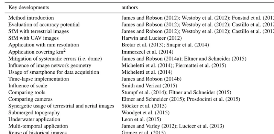
Table 3.Key developments of SfM photogrammetry towards a standard tool in geomorphometry.
Key developments authors
Method introduction James and Robson (2012); Westoby et al. (2012); Fonstad et al. (2013)
Evaluation of accuracy potential James and Robson (2012); Westoby et al. (2012); Castillo et al. (2012)
SfM with terrestrial images James and Robson (2012); Westoby et al. (2012); Castillo et al. (2012)
SfM with UAV images Harwin and Lucieer (2012)
Application with mm resolution Bretar et al. (2013); Snapir et al. (2014)
Application covering km2 Immerzeel et al. (2014)
Mitigation of systematic errors (i.e. dome) James and Robson (2014a); Eltner and Schneider (2015)
Influence of image network geometry Micheletti et al. (2014); Piermattei et al. (2015)
Usage of smartphone for data acquisition Micheletti et al. (2014)
Time-lapse implementation James and Robson (2014b)
Influence of scale Smith and Vericat (2015)
Comparing tools Stumpf et al. (2014); Eltner and Schneider (2015)
Comparing cameras Eltner and Schneider (2015); Prosdocimi et al. (2015)
Synergetic usage of terrestrial and aerial images Stöcker et al. (2015)
Submerged topography Woodget et al. (2015)
Underwater application Leon et al. (2015)
Multi-temporal application James and Varley (2012); Lucieer et al. (2013)
Reuse of historical images Gomez et al. (2015)
ing GUIs. Sf3M (Castillo et al., 2015) exploits VisualSfM and sfm_georef and additional CloudCompare command-line capacities for image-based surface reconstruction and subsequent point cloud editing within one GUI tool. Over-all, non-commercial applications have provided a wide range of SfM photogrammetry-related solutions that are constantly being improved on the basis of collaborative efforts. Com-mercial software packages are not further displayed due to their usual lack of detailed information regarding applied al-gorithms and their black box approach.
A variety of tools for SfM photogrammetry (at least 10 different) are used within the differing studies of this review (Fig. 3). Agisoft PhotoScan is by far the most employed soft-ware, which is probably due to its ease of use. However, this software is commercial and works on the black box princi-ple, which is in contrast to the second most popular tool, Bundler, in combination with PMVS or CMVS. The tool APERO in combination with MicMac focuses on accuracy instead of automation (Pierrot-Deseilligny and Clery, 2011), which is different to the former two. The high degree of pos-sible user–software interaction, which can be very advanta-geous to adopt the 3-D reconstruction to each specific case study, might also be its drawback because further knowledge into the method is required. Only a few studies have used the software in geoscientific investigations (Bretar et al., 2013; Stumpf et al., 2014; Ouédraogo et al., 2014; Stöcker et al., 2015; Eltner and Schneider, 2015).
3 Key developments in SfM photogrammetry
The vast recognition of SfM photogrammetry resulted in a large variety of its implementation leading to methodologi-cal developments, which have validity beyond its original
ap-plication. Thus, regarding geomorphometric investigations, studies considering the field of applications as well as eval-uations of the method’s performance induced key advances for SfM photogrammetry to establish as a standard tool in geosciences (Table 3). In the following, the approach is in-troduced concerning the selection and retrieval of scientific papers utilising SfM photogrammetry.
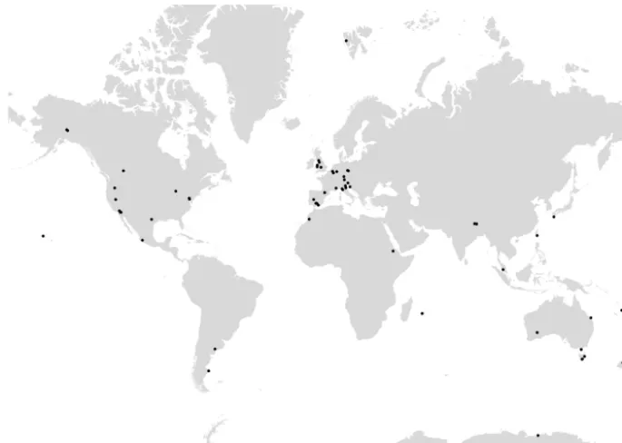
A survey of 65 scientific papers published between 2012 and 2015 was conducted, covering a wide range of applica-tions of SfM photogrammetry in geoscientific analysis (see Appendix A for a detailed list). Common scientific journals, academic databases and standard online searches have been used to search for corresponding publications. However, it has to be noted that our approach does not guarantee full cov-erage of the published works using SfM photogrammetry in geosciences. Nevertheless, various disciplines, locations and approaches from all continents are contained in this review (Fig. 2).
To put research hotspots in perspective, it should be taken into account that the number of publications in each disci-pline is not only dependent on the applicability of the method in that specific field of research. To a greater degree it is closely linked to the overall number of studies, which in the end can probably be broken down to the actual number of re-searchers in that branch of science. Relative figures revealing the relation between SfM photogrammetry-oriented studies to all studies of a given field of research would be desirable but are beyond the scope of this review.
Figure 2.Map of the research sites of all studies of this review.
Figure 3.Variety of SfM photogrammetry tools used in the 65 reviewed studies.
Different disciplines started to use SfM algorithms more or less simultaneously.
A list of all topics reviewed in this manuscript according to their year of appearance is shown in Table 4. It is impor-tant to note that most subjects are not strictly separable from each other: for instance, a heavy flash flood event will likely trigger heavy damage by soil erosion or upstream slope fail-ures. Thus, corresponding studies are arranged in regard to their major focus. The topic soil science comprises studies of soil erosion as well as soil microtopography.
3.1 Soil science
Table 4.Overview of the publication history divided into the main topics from 2012 until editorial deadline in November 2015. Several publications examined more than one topic, resulting in a larger number of topics than actual publications (number in brackets in last row). IDs refer to the table in Appendix A1.
Topic 2012 2013 2014 2015 2016 ID Total number
of publications on the respective topic
Soil
science/erosion
1 – 5 9 – 1, 2, 3, 5, 6, 9, 11,
18, 22, 23, 30, 31, 55, 60, 61
15
Volcanology 3 1 1 1 – 7, 15, 43, 44, 52,
54
6
Glaciology – – 4 6 – 12, 13, 14, 25,
27, 34, 37, 47, 51, 62
10
Mass movements – 1 1 3 – 32, 35, 49, 56, 64 5
Fluvial morpho-logy
– 1 5 3 1 4, 8, 16, 17, 21,
26, 29, 33, 37, 38
10
Coastal morpho-logy
3 1 3 – – 15, 20, 28, 36,
42, 50, 53
7
Others 1 2 8 5 – 7, 10, 17, 19, 24,
39, 40, 41, 45, 46, 48, 57, 58, 59, 63, 65
16
Topics 8 6 27 27 1 69
(publications) (6) (6) (25) (27) (1) (65)
camera-based surface reconstruction by combining indepen-dently captured terrestrial images with surface models from UAV images to fill data gaps and achieve a comprehensive 3-D model. Large areal coverage and very high resolution al-lowed for a new quality in the assessment of plot-based soil erosion analysis (Eltner et al., 2015)
Another six studies tackle the 3-D reconstruction of soil microtopography by producing very dense point clouds or DEMs. These data further serve to assess pros and cons of SfM photogrammetry, e.g. detection of small-scale erosion features (Nouwakpo et al., 2014), with regard to the doming effect (Eltner and Schneider, 2015) or as input parameter for erosion modelling (Kaiser et al., 2015).
3.2 Volcanology
Volcanology is a pioneering area of SfM photogrammetry re-search in geosciences because three out of six studies in 2012 included volcanic research sites. James and Robson (2012) acquired information on volcanic dome volume and struc-tural variability prior to an eruption from multi-temporal im-agery taken from a light aeroplane. Another interesting work by Bretar et al. (2013) successfully reveals roughness dif-ferences in volcanic surfaces from lapilli deposits to slabby pahoehoe lava.
3.3 Glaciology
Glaciology and associated moraines are examined in 7 pub-lications. In several UAV campaigns Immerzeel et al. (2014) detected limited mass losses and low surface velocities but high local variations of melt rates that are linked to supra-glacial ponds and ice cliffs. Rippin et al. (2015) present another UAV-based work on supra-glacial runoff networks, comparing the drainage system to surface roughness and sur-face reflectance measurements and detecting linkages be-tween all three. Furthermore, snow depth estimation and rock glacier monitoring are increasingly performed with SfM pho-togrammetry (Nolan et al., 2015; Dall’Asta et al., 2015).
3.4 Mass movements
for monitoring landslide displacements and erosion during several measuring campaigns, including the study of sea-sonal dynamics on the landslide body, superficial deforma-tion and rockfall occurrence. In addideforma-tion, these authors as-sessed the accuracy of two different 3-D reconstruction tools compared to lidar data.
3.5 Fluvial morphology
Channel networks in floodplains were surveyed by Pros-docimi et al. (2015) in order to analyse eroded channel banks and to quantify the transported material. Besides clas-sic DSLR cameras, evaluation of an iPhone camera revealed sufficient accuracy, so that in the near future non-scientists will also be able to carry out post-event documentation of damage. An interesting large-scale riverscape assessment is presented by Dietrich (2016), who carried out a helicopter-based data acquisition of a 32 km river segment. A small he-licopter proves to close the gap between unmanned platforms and commercial aerial photography from aeroplanes.
3.6 Coastal morphology
In the article by Westoby et al. (2012), several morphological features of contrasting landscapes were chosen to test the ca-pabilities of SfM, one of them being a coastal cliff of roughly
80 m height. Up to 90 000 points m−2enabled the
identifica-tion of bedrock faulting. Ruži´c et al. (2014) produced sur-face models of coastal cliffs to test the abilities of SfM pho-togrammetry in undercuts and complex morphologies.
3.7 Other fields of investigation in geosciences
In addition to the prevalent fields of attention, more exotic research is also being carried out, unveiling unexpected pos-sibilities for SfM photogrammetry. Besides the benefit for the specific research itself, these branches are important as they either explore new frontiers in geomorphometry or demon-strate the versatility of the method. Lucieer et al. (2014) analyse arctic moss beds and their health conditions by us-ing high-resolution surface topography (2 cm DEM) to sim-ulate water availability from snow melt. Leon et al. (2015) acquired underwater imagery of a coral reef to produce a DEM with a resolution of 1 mm for roughness estimation. Genchi et al. (2015) used UAV-image data of an urban cliff structure to identify bioerosion features and found a pattern in preferential locations.
The reconsideration of historical aerial images is another interesting opportunity arising from the new algorithmic image-matching developments that allow for new DEM res-olutions and thus possible new insights into landscape evolu-tion (Gomez et al., 2015).
4 Error assessment of SfM photogrammetry in
geoscientific applications
SfM photogrammetry has been tested under a large variety of environments due to the commensurate novel establishment of the method in geosciences, revealing numerous advan-tages but also disadvanadvan-tages regarding each application. It is important to have method-independent references to eval-uate 3-D reconstruction tools confidently. In total, 39 studies are investigated (Table A1) where a reference has been set up, either area-based (e.g. terrestrial laser scanning, TLS) or point-based (e.g. RTK GPS points). Because not all studies perform accuracy assessment with independent references, the number of studies is in contrast to the number of 65 stud-ies that are reviewed in regard to applications. In the follow-ing, methods are illustrated concerning integrated considera-tion of error performance of SfM photogrammetry in geosci-entific studies.
A designation of error parameters is performed prior to comparing the studies to avoid using ambiguous terms. There is a difference between local surface quality and more sys-tematic errors, i.e. due to referencing and project geome-try (James and Robson, 2012). Specifically, error can be as-sessed in regard to accuracy and precision.
Measurement accuracy, which defines the closeness of the measurement to a reference, ideally displays the true surface and can be estimated by the mean error value. However, pos-itive and negative deviations can compensate for each other and thus can impede the recognition of a systematic error (e.g. symmetric tilting) with the mean value. Therefore, nu-merical and spatial error distribution should also be consid-ered so as to investigate the quality of the measurement (e.g. Smith et al., 2015). For the evaluation of two DEMs, the iter-ative closest point (ICP) algorithm can improve the accuracy significantly if a systematic linear error (e.g. shifts, tilts or scale variations) is given, as demonstrated by Micheletti et al. (2014). Nevertheless, this procedure can also induce an error when the scene has changed significantly between the two data sets.
Precision, which defines the repeatability of the measure-ment (for example, it indicates how rough an actual planar surface is represented), usually comprises random errors that can be measured with the standard deviation or RMSE. How-ever, precision is not independent from systematic errors. In this study, the focus lies on RMSE or standard deviation cal-culated to a given reference (e.g. to a lidar point cloud) and thus the general term “measured error” is used.
Furthermore, error ratios are calculated to compare SfM photogrammetry performance between different studies un-der varying data acquisition and processing conditions.
Thereby, the relative error (er), the reference superiority (es)
and the theoretical error ratio (et) are considered. The first is
er=
σm
D, (1)
whereer is the relative error,σmthe measured error andD
the mean distance between the camera and surface.
The reference superiority displays the ratio between the measured error and the error of the reference (Eq. 2). It de-picts the validity of the reference to be accountable as a reli-able data set for comparison.
es=
σm
σref
, (2)
wherees is the reference superiority and σref the reference
error.
The theoretical error ratio includes the theoretical error, which is an estimate of the theoretically best achievable pho-togrammetric performance under ideal conditions. It is calcu-lated separately for convergent and parallel-axes image ac-quisition schemes. The estimate of the theoretical error of depth measurement for the parallel-axis case is displayed by Eq. (3) (more detail in Kraus, 2007). The error is determined for a stereo-image pair and thus might overestimate the er-ror for multi-view reconstruction. Basically, the erer-ror is in-fluenced by the focal length, the camera-to-surface distance and the distance between the images of the stereo-pair (base).
σp=
D2
Bcσi, (3)
whereσpis the coordinate error for parallel-axes case,cthe
focal length,σithe error image measurement andBthe
dis-tance between images (base).
For the convergent case the error also considers the camera-to-surface distance and the focal length. However, instead of the base the strength of image configuration de-termined by the angle between intersecting homologous rays is integrated and additionally the employed number of im-ages is accounted for (Eq. 4; more detail in Luhmann et al., 2014).
σc=
qD
√
kcσi, (4)
whereσc is the coordinate error for convergent case,q the
strength of image configuration, i.e. convergence, andk the
number of images.
Finally, the theoretical error ratio is calculated displaying the relation between the measured error and the theoretical error (Eq. 5). The value depicts the performance of SfM pho-togrammetry in regard to the expected accuracy.
et=
σm
σtheo
, (5)
whereetis the theoretical error ratio andσtheothe theoretical
error, eitherσporσc.
The statistical analysis of the achieved precisions of the reviewed studies is performed with the Python Data Analy-sis Library (pandas). If several errors are given in one study due to testing of different survey or processing conditions, the error value representing the enhancement of the SfM per-formance is chosen, i.e. in the study of Javernick et al. (2014) the DEM without an error dome, in the study of Rippin et al. (2015) the linear corrected DEM, and in the study of Eltner and Schneider (2015) the DEMs calculated with undistorted images. In addition, if several approaches are conducted to retrieve the deviation value to the reference, the more reliable error measure is preferred (with regard to Stumpf et al., 2014 and Gómez-Gutiérrez et al., 2014a and 2015). Apart from those considerations, measured er-rors have been averaged if several values are reported in one study, i.e. concerning multi-temporal assessments or consid-eration of multiple surfaces with similar characteristics, but not for the case of different tested SfM tools. Regarding data visualisation, outliers that complicated plot drawing were ne-glected within the concerning graphics. This concerned the study of Dietrich (2016) due to a very large scale of an in-vestigated river reach (excluded from Figs. 4a and 5a–b), the study of Snapir et al. (2014) due to a very high reference ac-curacy of Lego bricks (excluded from Figs. 4c and 5b), and the study of Frankl et al. (2015) due to a high measured er-ror as the study focus was rather on feasibility than accuracy (excluded from Fig. 5c).
Besides exploiting a reference to estimate the performance of the 3-D reconstruction, registration residuals of GCPs re-sulting from BA can be taken into account for a first error assessment. But this is not suitable as an exclusive error mea-sure due to potential deviations between the true surface and the calculated statistical and geometric model, which are not detectable with the GCP error vectors alone because BA is optimised to minimise the error at these positions. However, if BA has been performed in two stages (i.e. SfM and ref-erencing calculated separately), the residual vector provides reliable quality information because registration points are not integrated into model estimation.
Error evaluation in this study is performed with reference measurements. Thereby, errors due to the performance of the method itself and errors due to the method of quality assess-ment have to be distinguished.
4.1 Error sources of SfM photogrammetry
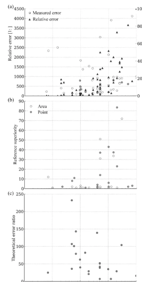
Figure 4.Box plots summarising statistics: (a) of the scale of the study reaches (N: 56; ID 1–3 and 5–39 in Appendix A), (b) the rel-ative error (calculated in regard to distance and measured error, N: 54; ID 1–3, 5–12 and 14–39 in Appendix A), and (c) the reference superiority (calculated in regard to measured error and reference er-ror, N: 33; ID 1–30 and 32–39 in Appendix A) of reviewed studies.
4.1.1 Scale and sensor to surface distance
SfM photogrammetry has the advantage of being useable at almost any scale. Thus, in the reviewed studies the method is applied at a large range of scales (Fig. 4a), reaching from 10 cm for volcanic bombs (Favalli et al., 2012; James and Robson, 2012) up to 10 km for a river reach (Dietrich, 2016). Median scale amounts to about 100 m. SfM photogrammetry reveals a scale-dependent practicability (Smith and Vericat, 2015) if case-study-specific tolerable errors are considered, e.g. for multi-temporal assessments. For instance, at plot and hillslope scale, 3-D reconstruction is a very sufficient method for soil erosion studies, even outperforming TLS (Nouwakpo et al., 2015; Eltner et al., 2015; Smith and Vericat, 2015). The method should be most useful in small-scale study reaches (Fonstad et al., 2013), whereas error behaviour is not as ad-vantageous for larger scales, i.e. catchments (Smith and Ver-icat, 2015).
Besides scale, the distance between sensor and surface is important for image-based reconstructed DEM error, also because scale and distance interrelate. The comparison of the reviewed studies indicates that with an increase in dis-tance the measured error increases, which is not unexpected (Fig. 5a, circles). However, there is no linear trend detectable. Therefore, the relative error is not assignable. The relative er-ror displays a large range from 15 to 4000 with a median of 400, thus revealing a rather low error potential (Fig. 5a, tri-angles). Very high ratios are solely observable for very close-range applications and at large distances. A general increase in the relative error with distance is observable (Fig. 5a, trian-gles). The indication that centimetre-accurate measurements are realisable at distances below 200 m (Stumpf et al., 2014) can be confirmed by Fig. 5a because most deviations are
low 10 cm up to that range. Overall, absolute error values are low at close ranges, whereas the relative error is higher at larger distances.
4.1.2 Camera calibration
SfM photogrammetry allows for straightforward handling of camera options due to integrated self-calibration, but knowl-edge about some basic parameters is necessary to avoid un-wanted error propagation into the final DEM from insuffi-ciently estimated camera models. The autofocus as well as automatic camera stabilisation options should be deactivated if a pre-calibrated camera model is used or one camera model is estimated for the entire image block because changes in the interior camera geometry due to camera movement can-not be captured with these settings. The estimation of a sin-gle camera model for one image block is usually preferable, if a single camera has been used, whose interior geometry is temporary stable, to avoid over-parameterisation (Pierrot-Deseilligny and Clery, 2011). Thus, if zoom lenses are moved a lot during data acquisition, they should be avoided due to their instable geometry (Shortis et al., 2006; Sanz-Ablanedo et al., 2010) that impedes usage of pre-calibrated fixed or single camera models. A good compromise between camera stability, sensor size and equipment weight, which is more relevant for UAV applications, is achieved by compact sys-tem cameras (Eltner and Schneider, 2015). However, solely three studies utilise compact system cameras in the reviewed studies (Tonkin et al., 2014; Eltner and Schneider, 2015; Elt-ner et al., 2015).
Along with camera settings, the complexity in regard to the considered parameters of the defined camera model within the 3-D reconstruction tool is relevant as well as the implementation of GCPs to function as further obser-vations in the BA, i.e. to avoid DEM domes as a conse-quence of insufficient image distortion estimation (James and Robson, 2014a; Eltner and Schneider, 2015). Also, Stumpf et al. (2014) detect worse distortion correction with a basic SfM tool, considering a simple camera model, compared to more complex software, integrating a variety of camera mod-els and GCP consideration. Camera calibration is a key ele-ment for high DEM quality, which is extensively considered in photogrammetric software, whereas simpler models that solely estimate principle distance and radial distortion are usually implemented in the SfM tools originating from com-puter vision (Eltner and Schneider, 2015; James and Robson, 2012; Pierrot-Deseilligny and Clery, 2011).
4.1.3 Image resolution
Image resolution is another factor influencing the final DEM quality. In particular, the absolute pixel size needs to be ac-counted for due to its relevance for the signal-to-noise ra-tio (SNR) because the larger the pixel the higher the amount of light that can be captured and hence a more distinct
sig-nal is measured. Resolution alone by means of pixel num-ber gives no information about the actual metric sensor size. A large sensor with large pixels and a large number of pix-els provides better image quality due to reduced image noise than a small sensor with small pixels but the same number of pixels. Thus, high image resolution defined by large pixel numbers and pixel sizes results in sufficient quality of images and thus DEMs (Micheletti et al., 2014; Eltner and Schnei-der, 2015).
However, the reviewed investigations indicate no obvious influence of the pixel size at the DEM quality. Mostly, cam-eras with middle-sized sensors and corresponding pixel sizes around 5 µm are used and a large range of errors at different pixel sizes is given.
To speed up processing, down-sampling of images is often performed, causing interpolation of pixels and thus the re-duction of image information, which can be the cause of un-derestimation of high-relief changes, e.g. observed by Smith and Vericat (2015) or Nouwakpo et al. (2015). Interestingly, Prosdocimi et al. (2015) reveal that lower errors are possi-ble with decreasing resolution due to an increase in error smoothing. Nevertheless, image data collection in the field should be done at highest realisable resolution and highest SNR to fully keep control over subsequent data process-ing – i.e. data smoothprocess-ing should be performed under self-determined conditions at the desktop, which is especially im-portant for studies of rough surfaces to allow for probate er-ror statistics (e.g. Brasington et al., 2012).
4.1.4 Image network geometry
In regard to the geometry of the image network, several pa-rameters are important: number of images, image overlap, obliqueness and convergence.
At least three images need to capture the area of interest, but for redundancy and to decrease DEM error, higher num-bers are preferred (James and Robson, 2012). For instance, Piermattei et al. (2015) detect better qualities for a higher number of images. However, the increase in images does not linearly increase the accuracy (Micheletti et al., 2014), and may ultimately lead to unnecessary increase in computation time. Generally, image number should be chosen depending on the size and complexity of the study reach (James and Robson, 2012), i.e. as high as possible but still keeping in mind acceptable processing time.
High image overlap is relevant to finding homologous points within many images that cover the entire image space. Stumpf et al. (2014) show that higher overlap resolves in better results. Wide-angle lenses whose radial distortion is within the limits should be chosen for data acquisition.
Ver-icat (2015) state that aerial images should be preferred if plots reach sizes larger than 100 m, because at these distances obliqueness of images becomes too unfavourable. Stumpf et al. (2014) even mention a distinct value of the incidence
an-gle of 30◦to the captured surface above which data quality
decreases significantly.
Furthermore, image network geometry has to be consid-ered separately for convergent acquisitions schemes, com-mon for terrestrial data collection, and for parallel-axes ac-quisition schemes, common for aerial data collection. The parallel-axes image configuration results in unfavourable er-ror propagation due to unfavourable parameter correlation, which inherits the separation between DEM shape and radial distortion (James and Robson, 2014a; Wu, 2014), resulting in a dome error that needs either GCP implementation or a well-estimated camera model for error mitigation (James and Robson, 2014a; Eltner and Schneider, 2015). However, GCP accuracy has to be sufficient or else the weight of GCP in-formation during BA is too low to avoid unfavourable corre-lations, as shown by Dietrich (2016), where DEM dome er-ror within a river reach could not be diminished even though GCPs were implemented into 3-D reconstruction. If conver-gent images are utilised, the angle of convergence is impor-tant, because the higher the angle, the better the image net-work geometry. Thereby, accuracy increases because suffi-cient image overlap is possible with larger bases between images. Therefore, glancing ray intersections, which impede distinct depth assignment, are avoided. But, at the same time, convergence should not be so high that the imaged scene becomes too contradictory for successful image matching (Pierrot-Deseilligny and Clery, 2012; Stöcker et al., 2015).
4.1.5 Accuracy and distribution of homologues image points
The quality of DEMs reconstructed from overlapping images depends significantly on the image-matching performance (Gruen, 2012). Image content and type, which cannot be en-hanced substantially, are the primary factors controlling the success of image matching (Gruen, 2012). Image matching is important for reconstruction of the image network geometry as well as the subsequent dense matching.
On the one hand, it is relevant to find good initial matches (e.g. SIFT features are not as precise as least-squares matches
with 1/10 pixel size accuracies; Gruen, 2012) to perform
re-liable 3-D reconstruction and thus retrieve an accurate sparse point cloud because optimisation procedures for model re-finement rely on this first point cloud. Thus, immanent errors will propagate along the different stages of SfM photogram-metry.
On the other hand, image-matching performance is more obviously important for dense reconstruction, when 3-D in-formation is calculated for almost every pixel. The accuracy of intersection during dense matching depends on the ac-curacy of the estimated camera orientations (Remondino et
al., 2014). If the quality of the DEM is the primary focus, which is usually not the case for SfM algorithms originat-ing from computer vision, the task of image matchoriginat-ing is still difficult (Gruen, 2012). Nevertheless, newer approaches are emerging, though, which still need evaluation in respect of accuracy and reliability (Remondino et al., 2014). An inter-nal quality control for image matching is important for DEM assessment (Gruen, 2012), but is mostly absent in tools for SfM photogrammetry.
So far, many studies exist which evaluate the quality of 3-D reconstruction in geoscientific applications. Nevertheless, considerations of dense-matching performance are still miss-ing, especially in regard to rough topographies (Eltner and Schneider, 2015).
4.1.6 Surface texture
Texture and contrast of the area of interest are significant to identify suitable homologous image points. Low textured and contrasted surfaces result in a distinct decrease in image features, i.e. snow-covered glaciers (Gómez-Gutiérrez et al., 2014a) or sandy beaches (Mancini et al., 2013). Furthermore, vegetation cover complicates image-matching performance due to its highly variable appearance from differing view-ing angles (e.g. Castillo et al., 2012; Eltner et al., 2015) and possible movements during wind. Thus, in this study, where present, only studies of bare surfaces are reviewed for error assessment.
4.1.7 Illumination condition
Ov and underexposure of images is another cause of er-ror in the reconstructed point cloud, which cannot be sig-nificantly improved by utilising high-dynamic-range (HDR) images (Gómez-Gutiérrez et al., 2015). Well-illuminated sur-faces result in a high number of detected image features, which is demonstrated for coastal boulders under varying light conditions by Gienko and Terry (2014). Furthermore, Gómez-Gutiérrez et al. (2014a) highlight the unfavourable influence of shadows because highest errors are measured in these regions; interestingly, these authors calculate the opti-mal time for image acquisition from the first DEM for multi-temporal data acquisition. Furthermore, the multi-temporal length of image acquisition needs to be considered during sunny conditions because with increasing duration shadow changes can decrease matching performance – i.e. with regard to the intended quality, surveys lasting more than 30 min should be avoided (Bemis et al., 2014). Generally, overcast but bright days are most suitable for image capture to avoid strong shadows or glared surfaces (James and Robson, 2012).
4.1.8 GCP accuracy and distribution
ground control for accurate DEM calculation, especially if one-staged BA is performed. In the common SfM workflow, integration of GCPs is less demanding because they are only needed to transform the 3-D model from the arbitrary co-ordinate system, which is comparable to the photogrammet-ric two-staged BA processing. A minimum of three GCPs are necessary to account for model rotation, translation and scale. However, GCP redundancy, i.e. more points, has been shown to be preferable to increase accuracy (James and Rob-son, 2012). A high number of GCPs further ensures the con-sideration of checkpoints not included for the referencing, which are used as independent quality measure of the final DEM. More complex 3-D reconstruction tools either expand the original 3-D Helmert transformation by secondary re-finement of the estimated interior and exterior camera ge-ometry to account for non-linear errors (e.g. Agisoft Photo-Scan) or integrate the ground control into the BA (e.g. AP-ERO). For instance, Javernick et al. (2014) were able to re-duce the height error to decimetre level by including GCPs in the model refinement.
Natural features over stable areas, which are explicitly identifiable, are an alternative for GCP distributions, al-though they usually lack strong contrast (as opposed to ar-tificial GCPs) that would allow for automatic identification and sub-pixel accurate measurement (e.g. Eltner et al., 2013). Nevertheless, they can be suitable for multi-temporal change detection applications, where installation of artificial GCPs might not be possible (e.g. glacier surface reconstruction; Piermattei et al., 2015) or necessary as in some cases rel-ative accuracy is preferred over absolute performance (e.g. observation of landslide movements; Turner et al., 2015).
GCP distribution needs to be even and adapted to the ter-rain resulting in more GCPs in areas with large changes in relief (Harwin and Lucieer, 2012) to cover different terrain types. Harwin and Lucieer (2012) state an optimal GCP
dis-tance between 1/5 and 1/10 of object distance for UAV
applications. Furthermore, the GCPs should be distributed widely across the target area (Smith et al., 2015) and at the edge or outside the study reach (James and Robson, 2012) to enclose the area of interest, because if the study area is extended outside the GCP area, a significant increase in er-ror is observable in that region (Smith et al., 2014; Javernick et al., 2014; Rippin et al., 2015). If data acquisition is per-formed with parallel-axis UAV images and GCPs are imple-mented for model refinement, rules for GCP setup according to classical photogrammetry apply, i.e. dense GCP installa-tion around the area of interest and height control points in specific distances as function of image number (more detail in e.g. Kraus, 2007).
The measurement of GCPs can be performed within either the point cloud or the images, preferring the latter because identification of distinct points in 3-D point clouds of vary-ing density can be less reliable (James and Robson, 2012; Harwin and Lucieer, 2012) compared to sub-pixel measure-ment in 2-D images, where accuracy of GCP identification
basically depends on image quality. Figure 5a illustrates that only a few studies have measured GCPs in point clouds, re-sulting higher errors compared to other applications at the same distance.
4.2 Errors due to accuracy/precision assessment technique
4.2.1 Reference of superior accuracy
It is difficult to find a suitable reference for error assess-ment of SfM photogrammetry in geoscientific or geomor-phologic applications due to the usually complex and rough nature of the studied surfaces. So far, either point-based or area-based measurements have been carried out. On the one hand, point-based methods (e.g. RTK GPS or total station) ensure superior accuracy but lack sufficient area coverage for precision statements of local deviations; on the other hand, area-based (e.g. TLS) estimations are used, which provide enough data density but can be lacking in sufficient accu-racy (Eltner and Schneider, 2015). Roughness is the least constrained error within point clouds (Lague et al., 2013) in-dependent from the observation method. Thus, it is difficult to distinguish between method noises and the actual signal of method differences, especially at scales where the reference method reaches its performance limit. For instance, Tonkin et al. (2014) indicate that the quality of total station points is not necessarily superior on steep terrain.
Generally, 75 % of the investigations reveal a measured er-ror that is 20 times higher than the erer-ror of the reference. But the median shows that the superiority of the reference ac-curacy is actually significantly poorer; the measured error is merely twice the reference error (Fig. 4c). The reviewed stud-ies further indicate that the superior accuracy of the reference seems to depend on the camera-to-object distance (Fig. 5b). At shorter distances (below 50 m) most references reveal ac-curacies that are lower than one magnitude superiority to the measured error. However, alternative reference methods are still absent. For applications solely in further distances the references are sufficient. These findings are relevant for the interpretation of the relative error because low ratios at small-scale reaches might be due to the low performance of the reference rather than the actual 3-D reconstruction quality, but due to the reference noise lower errors they are not de-tectable. Low relative errors are measured where the supe-rior accuracy is also low (distance 5–50 m) and large ratios are given at a distance where superior accuracy increases as well.
4.2.2 Type of deviation measurement
the application of raster inherits the disadvantage of data in-terpolation, especially relevant for rough surfaces or com-plex areas (e.g. undercuts as demonstrated for gullies by Frankl et al., 2015). In this context it is important to note that lower errors are measured for point-to-point distances rather than raster differencing (Smith and Vericat, 2015; Gómez-Guiérrez et al., 2014b).
Furthermore, within 3-D evaluation, different methods for deviation measurement exist. The point-to-point comparison is solely suitable for a preliminary error assessment because this method is prone to outliers and differing point densities. By point cloud interpolation alone (point-to-mesh), this is-sue is not solvable because there are still problems at very rough surfaces (Lague et al., 2013). Different solutions have been proposed: on the one hand, Abellán et al. (2009) pro-posed averaging the point cloud difference along the
spa-tial dimension, which can also be extended to 4-D (x, y,
z, time; Kromer et al., 2015). On the other hand, Lague et
al. (2013) proposed the M3C2 algorithm for point cloud parison that considers the local roughness and further com-putes the statistical significance of detected changes. Stumpf et al. (2014) and Gómez-Gutiérrez et al. (2015) illustrated lower error measurements with M3C2 compared to point-to-point or point-to-point-to-mesh. Furthermore, Kromer et al. (2015) showed how the 4-D filtering, when its implementation is feasible, allows for a considerably increase in the level of detection compared to other well-established techniques of comparison.
4.3 Standardised error assessment
To compare the achieved accuracies and precisions of dif-ferent studies a standardised error assessment is necessary, e.g. considering the theoretical error ratio. The calculation of the theoretical error for the convergent image acquisition schemes is possible, making some basic assumptions about the network geometry, i.e. the strength of image configura-tion equals 1 (as in James and Robson, 2012), the number of images equals 3 (as in James and Robson, 2012) and an image measurement error of 0.29 due to quantisation noise (as a result of continuous signal conversion to discrete pixel value). However, it is not possible to evaluate the theoret-ical error for parallel-axes case studies because informa-tion about the distance between subsequent images (base) is mostly missing but essential to solve the equation and should not be assumed. Eltner and Schneider (2015) and Eltner et al. (2015) compare their results to parallel-axes theoretical error and demonstrate that photogrammetric accuracy is at least possible for soil surface measurement from low flying heights (e.g. sub-centimetre error for altitudes around 10 m). The results from James and Robson (2012), which show a less reliable performance of SfM than expected from photogrammetric estimation, can be confirmed by the re-viewed studies. Image-based 3-D reconstruction, considing SfM workflows, performs poorer than the theoretical
er-ror (Fig. 5c). The measured erer-ror is always higher and on average 90 times worse than the theoretical error. Even for the smallest theoretical error ratio the actual error is 6 times higher. Furthermore, it seems that with increasing distance theoretical and measured errors converge slightly.
As demonstrated, diverse factors influence SfM pho-togrammetry performance and subsequent DEM error with different sensitivity. Generally, accurate and extensive data acquisition is necessary to minimise error significantly (Jav-ernick et al., 2014). Independent reference sources, such as TLS, are not replaceable (James and Robson, 2012) due to their differing error properties (i.e. error reliability) com-pared to image matching (Gruen, 2012). Synergetic effects of SfM and classical photogrammetry should be used, i.e. benefiting from the high automation of SfM to retrieve initial estimates without any prior knowledge about the image scene and acquisition configuration and adjacent reducing error by approved photogrammetric approaches which are optimised for high accuracies.
The reviewed studies indicate the necessity of a standard-ised protocol for error assessment because the variety of stud-ies inherit a variety of scales worked at, software used, GCP types measured, deviation measures applied, image network configurations implemented, cameras and platforms operated and reference utilised, making it very difficult to compare results with consistency. Relevant parameters for a standard protocol are suggested in Fig. 6.
5 Perspectives and limitations
stud-Figure 6.Data acquisition and error assessment protocol for SfM photogrammetry, independent of individual study design.
ies during the next decade; perspectives include efforts in cross-disciplinarity, process automation, data and code shar-ing, real-time data acquisition and processshar-ing, unlocking the archives, etc., as follows.
5.1 Cross-disciplinarity
A great potential relies on adapting three-dimensional meth-ods originally developed for the treatment of 3-D lidar data to investigate natural phenomena through SfM photogram-metry techniques. Applications on 3-D point cloud treatment dating back to the last decade will soon be integrated into SfM photogrammetry post-processing; examples include ge-omorphological investigations in high-mountain areas (Mi-lan et al., 2007), geological mapping (Buckley et al., 2008; Franceschi et al., 2009), soil erosion studies (Eltner and Baumgart, 2015), investigation of fluvial systems (Heritage and Hetherington, 2007; Cavalli et al., 2008; Brasington et al., 2012), and mass wasting phenomena (Lim et al., 2005; Oppikofer et al., 2009; Abellán et al., 2010).
the usage of mobile systems (Lato et al., 2009; Michoud et al., 2015).
5.2 Data and code sharing
Open data in geomorphometric studies using point clouds are also needed. The development of open-source software for handling huge 3-D data sets such as CloudCompare (Girardeau-Montaut, 2015) has considerably boosted geo-morphometric studies using 3-D point clouds due to provid-ing facile processprovid-ing of such memory-intense data. Neverthe-less, apart from the above-mentioned case, sharing the source code or the RAW data of specific applications for investi-gating earth surface processes is still not well established in our discipline. A series of freely available databases exist for lidar data sets (www.openTopography.org, www.rockbench. org, http://3d-landslide.com/). However, to the knowledge of the authors, there is no specific GitHub cluster or website dedicated to the maintaining and development of open-access software in geosciences.
5.3 Unlocking the archive
The appraisal of digital photography and the exponential in-crease in data storage capabilities have enabled the existence of the massive archive of optical images around the world. Accessing such quantity of information could provide unex-pected opportunities for the four-dimensional research of ge-omorphological processes using SfM photogrammetry work-flows. Except for some open repositories (e.g. Flickr, Google Street View) the possibility to access the massive optical data is still scarce. In addition, accessing such databases may be-come a challenging task due to data interchangeability issues. A considerable effort may be necessary for creating such a database with homogeneous data formats and descriptors (type of phenomenon, temporal resolution, pixel size, accu-racy, distance to object, existence of GCPs, etc.) during the coming years.
A first valuable approach to use data from online imagery was presented by Martin-Brualla et al. (2015), who pave the way for further research in a new field of 3-D surface analysis (i.e. time lapse). Other possible applications might unlock archives of historical airborne, helicopter-based or terrestrial imagery, ranging from the estimation of coastal retreat rates to the observation of the evolution of natural hazards to the monitoring of glacier fronts, and further.
5.4 Real-time data acquisition
Rapid developments in automation (soft- and hardware wise) allow for in situ data acquisition and its immediate transfer to processing and analysing institutions. Thus, extreme events are recognisable during their occurrence and authorities or rescue teams can be informed in real time. In this context SfM photogrammetry could help to detect and quantify rapid
volume changes of, for example, glacier fronts, pro-glacial lakes, rock failures and ephemeral rivers.
Furthermore, real-time crowd sourcing offers an entirely new dimension of data acquisition. Due to the high connec-tivity of the public through smartphones, various possibilities arise to share data (Johnson-Roberson et al., 2015). An al-ready implemented example is real-time traffic information. Jackson and Magro (2015) name further options. Crowd-sourced imagery can largely expand possibilities to 3-D in-formation.
5.5 Time-lapse photography
A limited frequency of data acquisition increases the likeli-hood of superimposition and coalescence of geomorpholog-ical processes (Abellán et al., 2014). Since time-lapse SfM photogrammetry data acquisition has remained so far unex-plored, this topic is expected to be a great prospect during the coming years. To date, solely James and Robson (2014b) have demonstrated its potential by monitoring a lava flow at minute intervals for 37 min. One reason why time-lapse SfM photogrammetry remains rather untouched in geosciences lies in the complex nature of producing continuous data sets. Besides the need for an adequate research site (frequent morphodynamic activity), other aspects have to be taken into account: an automatic camera setup is required with self-contained energy supply (either via insolation or wind), adequate storage and appropriate choice of viewing angles onto the area of interest. Furthermore, cameras need to com-prise sufficient image overlap and have to be synchronised. Ground control is required and an automatic pipeline for large data treatment should be developed.
New algorithms are necessary to deal with massive point cloud databases. Thus, innovative four-dimensional ap-proaches have to be developed to take advantage of the infor-mation contained in real-time and/or time-lapse monitoring. Furthermore, handling huge databases is an important issue and although fully automatic techniques may not be neces-sary in some applications, a series of tedious and manual pro-cesses are still required for data treatment. Combining real-time and/or real-time-lapse data sets with climatic information can improve the modelling of geomorphological processes.
5.6 Automatic UAV surveying
However, a large limitation for such a realisation lies in legal restrictions, because national authorities commonly request that visual contact to the UAV be maintained in case of fail-ure. However, in remote areas installation of an automatic system could already be allowed by regulation authorities.
5.7 Direct geo-referencing
The use of GCPs is very time-consuming in the current SfM workflow. At first, a great deal of field efforts are needed to install and measure the GCPs during data acquisition. Af-terwards, more time and labour are required during post-processing in order to identify the GCPs in the images, al-though some progress is being made regarding to automatic GCP identification, e.g. by the exploitation of templates (Chen et al., 2000). The efficiency of geo-referencing can be increased significantly by applying direct geo-referencing. Thus, the location and position of the camera is measured in real time and synchronised to the image capture by an on-board GPS receiver and an IMU (inertial measurement unit) recording camera tilts. This applies to UAV systems as well as terrestrial data acquisition, e.g. by smartphones (Masiero et al., 2014). Exploiting direct geo-referencing can reduce usage of GCPs to a minimum or even replace it, which has already been demonstrated by Nolan et al. (2015), who
gen-erated DEMs with spatial extents of up to 40 km2and a
geo-location accuracy of±30 cm.
The technique can be very advantageous when it comes to monitoring areas with great spatial extents or inaccessible research sites. However, further development is necessary, thereby focusing on lightweight but precise GPS receivers and IMU systems, on UAVs due to their limited payload, and on hand-held devices due to their feasibility (e.g. Eling et al., 2015).
6 Conclusions
This review has shown the versatility and flexibility of the recently established method SfM photogrammetry. Due to its beneficial qualities, a wide community of geoscientists starts to implement 3-D reconstruction based on images within a variety of studies. To summarise the publications, there
are no considerable disadvantages mentioned (e.g. accuracy-wise) compared to other methods that cannot be counteracted by placement of GCPs, camera calibration or a high num-ber of images. Frontiers in geomorphometry have been ex-panded once more, as limits of other surveying techniques such as restricted mobility, isolated area of application and high costs are overcome by SfM photogrammetry. Its ma-jor advantages lie in easy-to-handle and cost-efficient digital cameras as well as non-commercial software solutions.
SfM photogrammetry is already becoming an essential tool for digital surface mapping. It is employable in a fully automatic manner, but individual adjustments can be con-ducted to account for each specific case study constraint and accuracy requirement in regard to the intended application. Due to the possibility of different degrees of process interac-tion, non-experts can utilise the method depending on their discretion.
While research of the last years has mainly focused on testing the applicability of SfM photogrammetry in various geoscientific applications, recent studies have tried to pave the way for future usages and develop new tools, setups or algorithms. Performance analysis has revealed the suitability of SfM photogrammetry at a large range of scales in regard to case-study-specific accuracy necessities. However, differ-ent factors influencing final DEM quality still need to be ad-dressed. This should be performed under strict experimental (laboratory) designs because complex morphologies, typical in earth surface observations, impede accuracy assessment due to missing superior reference. Thus, independent refer-ences and GCPs are still needed in SfM photogrammetry for reliable estimation of the quality of each 3-D reconstructed surface.
T ab le A1. Continued. ID Author Y ear Application Softw are Perspecti v e Distance [m] Scale* [m] Pix el size [µm] Image number Comple xity of SfM tool
Measure- ment error [mm]
Relati
v
e
error
Reference superi- ority Theo- retical error ratio
12 Gómez- Gutiérrez et al. 2014 rock glacier 123-D Catch terrestrial 300 130 8.2 6 basic 430 698 72 103 13 Gómez- Gutiérrez et al. 2015 rock glacier 123-D catch, PhotoScan terrestrial 300 130 8.2 9 basic, comple x 84–1029 – – – 14 Immerzeel et al. 2014 dynamics of debris-co v ered glacial tongue PhotoScan U A V 300 3500 1.3 284, 307 comple x 330 909 – – 15 James and Robson 2012 v olcanic bomb, sum-mit crater , coastal clif f Bundler + PMVS2
terrestrial, UA
V 0.7–1000 0.1– 1600 5.2 , 7.4 133– 210 basic 1000– 2333 0–62 1–12 16–25 16 Ja v ernick et al. 2014
braided riv
T ab le A1. Continued. ID Author Y ear Application Softw are Perspecti v e Distance [m] Scale* [m] Pix el size [µm] Image number Comple xity of SfM tool
Measure- ment error [mm]
Relati
v
e
error
Reference superi- ority Theo- retical error ratio
35 T urner et al. 2015
landslide change detection
PhotoScan U A V 40 125 4.3 62–415 comple x 31–90 444– 1290 1–3 – 36 W estoby et al. 2012 coastal clif f SfMT oolkit terrestria l 15 300 4.3 889 basic 500 100 – – 37 W estoby et al. 2014 moraine dam, allu-vial debris fan SfMT oolkit3 terrestrial 500 500 4.3 1002, 1054 basic 814, 85 614, 1176 2, 43 – 38 W oodget et al. 2015 fluvial topograph y PhotoScan U A V 26–28 50, 100 2.0 32–64 comple x 19–203 138– 1421 – – 39 Zarco-T ejada et al. 2014 tree height estimation Pix4-D U A V 200 1000 4.3 1409 comple x 350 571 23 – 40 Bemis et al. 2014 structural geology PhotoScan U A V , ter -restrial – – – – – – – – – 41 Bendig et al. 2013 crop gro wth PhotoScan U A V 30 7 – – – – – – – 42 Bini et al. 2014 coast ero-sion/abrasion Bundler terrestrial – – – – – – – – – 43 Bretar et al. 2013 (v olcanic) surf ace roughness APER O + MicMac terrestrial 1.5 5.9– 24.6 – – – – – – – 44 Brothelande et al. 2015
post- caldera resur
T
ab
le
A1.
Continued.
ID
Author
Y
ear
Application
Softw
are
Perspecti
v
e
Distance [m] Scale* [m]
Pix
el
size [µm] Image number
Comple
xity
of
SfM
tool
Measure- ment error [mm]
Relati
v
e
error
Reference superi- ority Theo- retical error ratio
63
T
orres-Sánchez
et
al.
2015
tree
planta-tion
PhotoScan
U
A
V
50,
100
–
–
–
–
–
–
–
–
64
T
urner
et
al.
2015
landslide monitoring
Bundler
+
PMVS2
U
A
V
50
–
–
–
–
–
–
–
–
65
V
asuki
et
al.
2014
structural geology
Bundler
+
PMVS2
U
A
V
30–40
100
–
–
–
–
–
–
–
ID
1–39:
these
studies
are
considered
for
error
performance
analysis.
Italic
te
xt:
for
most
authors
not
all
camera
parameters
are
gi
v
en.
Hence,
camera
parameters
are
retrie
v
ed
from
dpre
vie
w
.com
(or
similar
sources).
*If
scale
or
distance
is
not
gi
v
en,
it
is
estimated
from
study
area
display