Shapes for the Hazard Rate
T. H. M. Abouelmagd
Management Information System Department, Taibah University, Saudi Arabia
Department of Statistics, Mathematics and Insurance Benha University, Egypt
M. S. Hamed
Management Information System Department, Taibah University, Saudi Arabia
Department of Statistics, Mathematics and Insurance Benha University, Egypt
Ahmed Z. Afify
Department of Statistics, Mathematics and Insurance Benha University, Egypt
Abstract
We define and study a new continuous distribution called the exponentiated Weibull Burr XII. Its density function can be expressed as a linear mixture of Burr XII. Its hazard rate is very flexibile in accomodating various shapes including constant, decreasing, increasing, J-shape, unimodal or bathtub shapes. Various of its structural properties are investigated including explicit expressions for the ordinary and incomplete moments, generating function, mean residual life, mean inactivity time and order statistics. We adopted the maximum likelihood method for estimating the model parameters. The flexibility of the new family is illustrated by means of a real data application.
Keywords: Burr XII Distribution, Exponentiated Weibull-H family, Generating Function, Maximum Likelihood.
1. Introduction
(2017), the odd Lindley BXII distribution due to Abouelmagd et al. (2017) and the Kumaraswamy exponentiated BXII distribution defined by Mead and Afify (2017).
In this paper, we define and study a new five-parameter model named the exponentiated Weibull Burr XII (EWBXII) distribution which extends the WBXII distribution (Afify et al., 2017) and provide greater flexibility in modelling data. Based on the exponentiated Weibull-H (EW-H) family proposed by Cordeiro et al. (2017), we construct our newly model.
Consider the bsaeline cumulative distribution function (CDF) 𝐻(𝑥; 𝝃) with parameter vector 𝝃. Then, the CDF of the EW-H family is given by
𝐹(𝑥; 𝜈, 𝑎, 𝑏, 𝝃) = {1 − exp [−𝑎 ( 𝐻(𝑥;𝝃)
1−𝐻(𝑥;𝝃)) 𝑏
]}
𝜈
. (1)
The probability density function (PDF) of the EW-H family is
𝑓(𝑥; 𝜈, 𝑎, 𝑏, 𝝃) = 𝑎𝑏𝜈ℎ(𝑥; 𝝃) 𝐻(𝑥;𝝃)𝑏−1
[1−𝐻(𝑥;𝝃)]𝑏+1 exp [−𝑎 (
𝐻(𝑥;𝝃) 1−𝐻(𝑥;𝝃))
𝑏
]
× {1 − exp [−𝑎 ( 𝐻(𝑥;𝝃)
1−𝐻(𝑥;𝝃)) 𝑏
]}
𝜈−1
, (2)
where 𝜈, 𝑎 and 𝑏 are three additional positive shape parameters which provide greater flexibility in accommodating all forms of the hazard rate function (HRF).
The EWBXII distribution is a flexible model which exhibit all forms of the hazard rate function (HRF) as shown in Figure 2. Further, the EWBXII distribution contains seventeen sub-models as special cases.
The rest of the paper is outlined as follows. In Section 2, we define the EWBXII distribution, present its special models and provide some plots of its PDF and HRF. In Section 3, we derive a linear representation for the EWBXII PDF and obtain some of its mathematical properties including ordinary and incomplete moments, mean residual life, mean inactivity time, moment generating function (mgf) and order statistics. In Section 4, we use maximum likelihood to estimate the model parameters. In Section 5, we use a real data set to prove empirically the flexibility of the new model. Finally, some concluding remarks are given in Section 6.
2 The EWBXII distribution
In this section, we define the EWBXII distribution, provide its special cases and give some plots for its PDF and HRF.
The CDF and PDF of the two parameter BXII distribution are given by (for 𝑥 > 0)
𝐻(𝑥; 𝛼, 𝛽) = 1 − (1 + 𝑥𝛼)−𝛽 and ℎ(𝑥; 𝛼, 𝛽) = 𝛼𝛽𝑥𝛼−1(1 + 𝑥𝛼)−𝛽−1,
By inserting the CDF of the BXII in equation (1), we obtain the CDF of the EWBXII distribution
𝐹(𝑥) = (1 − exp {−𝑎[(1 + 𝑥𝛼)𝛽− 1]𝑏})𝜈, 𝑥 > 0
(3)
and the corresponding PDF of (3) is given by
𝑓(𝑥) = 𝑎𝑏𝜈𝛼𝛽𝑥𝛼−1 [1−(1+𝑥𝛼)−𝛽]
𝑏−1
(1+𝑥𝛼)−𝛽𝑏+1 exp {−𝑎[(1 + 𝑥
𝛼)𝛽− 1]𝑏}
× (1 − exp {−𝑎[(1 + 𝑥𝛼)𝛽− 1]𝑏})𝜈−1, (4)
where 𝛼, 𝛽, 𝑎, 𝑏 and 𝜈 are positive shape parameters which can provide more flexibility to model various real world data.
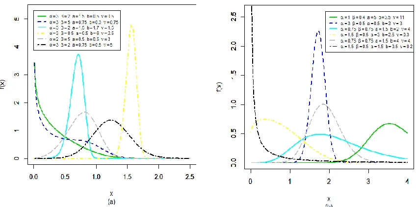
Plots of the PDF and HRF of the EWBXII distribution are displayed in Figures 1 and 2, respectively. The plots in Figure 1 show that the PDF of the EWBXII distribution can be reversed J-shape, right-skewed, left-skewed, symmetric or concave down. Figure 2 shows that the HRF of the proposed model can be constant, decreasing, increasing, J-shape, unimodal, bathtub shapes.
Figure 2: Some possible shapes for the EWBXII HRF
The EWBXII distribution is a comprehensive distribution which contains several lifetime models, such as Weibull BXII, exponential BXII (ExBXII), odd generalized exponential BXII (OGEx-BXII), Burr X BXII (BX-BXII), BXII, Lomax (Lo) and log logistic (LL) distributions as special cases. Table 1 provides all sub-models of the EWBXII distribution.
Table 1: Special cases of the EWBXII Distribution
No. Model 𝛼 𝛽 𝑎 𝑏 𝜈 Author
1 WBXII 𝛼 𝛽 𝑎 𝑏 1 Afify et al. (2017)
2 W Lomax 1 𝛽 𝑎 𝑏 1 -
3 W log-logistic 𝛼 1 𝑎 𝑏 1 -
4 Ex BXII 𝛼 𝛽 𝑎 1 1 -
5 Ex Lomax 1 𝛽 𝑎 1 1 -
6 Ex log-logistic 𝛼 1 𝑎 1 1 -
7 EW Lomax 1 𝛽 𝑎 𝑏 𝜈 New
8 EW log-logistic 𝛼 1 𝑎 𝑏 𝜈 New
9 OGEx-BXII 𝛼 𝛽 𝑎 1 𝜈 New
10 OGEx-Lomax 1 𝛽 𝑎 1 𝜈 New
11 OGEx-log-logistic 𝛼 1 𝑎 1 𝜈 New
12 BX-BXII 𝛼 𝛽 1 2 𝜈 New
13 BX- Lomax 1 𝛽 1 2 𝜈 New
14 BX- log-logistic 𝛼 1 1 2 𝜈 New
15 BXII 𝛼 𝛽 1 1 1 Burr (1942)
16 Lomax 1 𝛽 1 1 1 -
3. Some EWBXII properties
Some properties of the EWBXII distribution including ordinary and incomplete moments, generating function, mean residual life (MRL), mean inactivity time (MIT) and order statistics are derived in this section.
3.1 Linear representation
According to equation (4.5) in Cordeiro et al. (2017), the PDF of the EWBXII distribution can be rewritten as
𝑓(𝑥) = ∑
∞
𝑖,𝑘,𝑗=0
(−1)𝑘+𝑖𝜈𝑏𝑎𝑘+1(𝑖 + 1)𝑘Γ(𝜈)Γ([𝑘 + 1]𝑏 + 𝑗 + 1)
𝑖! 𝑘! 𝑗! Γ(𝜈 − 𝑖)Γ([𝑘 + 1]𝑏 + 1)
×𝛼𝛽𝑥𝛼−1(1 + 𝑥𝛼)−𝛽−1[1 − (1 + 𝑥𝛼)−𝛽](𝑘+1)𝑏+𝑗−1.
Applying the generalized binomial expansion to the last term, we have
𝑓(𝑥) = ∑∞𝑚=0 𝜙𝑚 𝑔𝛽(𝑚+1)(𝑥), (5)
where the constant term is given by
𝜙𝑚 = ∑
∞
𝑖,𝑘,𝑗=0
(−1)𝑘+𝑖+𝑚𝜈𝑏𝑎𝑘+1(𝑖 + 1)𝑘Γ(𝜈)Γ([𝑘 + 1]𝑏 + 𝑗)Γ([𝑘 + 1]𝑏 + 𝑗 + 1)
𝑖! 𝑘! 𝑗! (𝑚 + 1)! Γ(𝜈 − 𝑖)Γ([𝑘 + 1]𝑏 + 1)Γ([𝑘 + 1]𝑏 + 𝑗 − 𝑚)
and 𝑔𝛽(𝑚+1)(𝑥) refer to the BXII PDF with parameters 𝛼 and 𝛽(𝑚 + 1). Equation (5) is important in deriving some properties of the EWBXII distributions from those of the BXII distribution.
3.2 Moments
The 𝑟th ordinary moment of 𝑋, follows from (5) (for 𝛼𝛽(𝑚 + 1) > 𝑟) as
𝜇𝑟′ = ∑ ∞
𝑚=0
𝜙𝑚 𝛽(𝑚 + 1) 𝐵 (𝛽(𝑚 + 1) −
𝑟 𝛼,
𝑟 𝛼+ 1).
The mean of 𝑋 follows by setting 𝑟 = 1 in the above equation.
The 𝑟th incomplete moment of the EWBXII distribution follows from (5) as
𝜑𝑟(𝑡) = ∑
∞
𝑚=0
𝜙𝑚 𝛽(𝑚 + 1) 𝐵 (𝑡𝛼; 𝛽(𝑚 + 1) − 𝑟
When 𝒓 = 𝟏, we have the first incomplete moment of 𝑿
𝜑1(𝑡) = ∑
∞
𝑚=0
𝜙𝑚 𝛽(𝑚 + 1) 𝐵 (𝑡𝛼; 𝛽(𝑚 + 1) −1 𝛼,
1 𝛼+ 1)
which is important to calculate the Bonferroni and Lorenz curves and the MRL and MIT.
The MRL or life expectancy at age 𝑡 is defined by
𝑚𝑋(𝑡) =1 − 𝜑1(𝑡) 1 − 𝐹(𝑡) − 𝑡.
Using 𝜑1(𝑡), we obtain
𝑚𝑋(𝑡) =
1
1 − 𝐹(𝑡)∑
∞
𝑚=0
𝜙𝑚 𝛽(𝑚 + 1) 𝐵 (𝑡𝛼; 𝛽(𝑚 + 1) −
1 𝛼,
1
𝛼+ 1) − 𝑡.
The MIT is defined (for 𝑡 > 0) by
𝑀𝑋(𝑡) = 𝑡 −𝜑1(𝑡) 𝐹(𝑡)
By inserting 𝜑1(𝑡) in the above equation, we have the MIT of 𝑋 as
𝑀𝑋(𝑡) = 𝑡 −
1 𝐹(𝑡)∑
∞
𝑚=0
𝜙𝑚 𝛽(𝑚 + 1) 𝐵 (𝑡𝛼; 𝛽(𝑚 + 1) −
1 𝛼,
1 𝛼+ 1).
The mgf of𝑋 follows from (5) as
𝑀𝑋(𝑡) = ∑∞
𝑚=0 𝜙𝑚 𝑀𝛽(𝑚+1)(𝑡), (6)
where 𝑀𝛽(𝑚+1)(𝑡) is the mgf of the BXII distribution with two parameters 𝛼 and
𝛽(𝑚 + 1). Paranaíba et al. (2011) provided a simple formula for the mgf of BXII distribution with two-parameter 𝛼 and 𝛽 (for 𝑡 < 0) as
𝑀(𝑡) = 𝑠 𝐼 (−𝑡,𝑠
𝛽− 1, 𝑠
𝛽, −𝛽 − 1). (7)
Combining equations (6) and (7), the mgf of 𝑋 reduces to
𝑀𝑋(𝑡) = 𝑠 ∑
∞
𝑚=0
𝜙𝑚 𝐼 (−𝑡, 𝑠
𝛽(𝑚 + 1)− 1, 𝑠
3.3 Order statistics
Let 𝑋1, … , 𝑋𝑛 be a random sample of size 𝑛 from the EWBXII distribution and let
𝑋(1), … , 𝑋(𝑛) be the corresponding order statistics. Then, the pdf of the 𝑖th order statistic,
𝑋𝑖:𝑛, is given by
𝑓𝑖:𝑛(𝑥) = 𝑛!𝑓(𝑥)
(𝑖−1)!(𝑛−𝑖)!∑ 𝑛−𝑖
𝑗=0 (−1)𝑗(𝑛−𝑖𝑗 ) 𝐹(𝑥)𝑗+𝑖−1. (8)
Based on equation (6.2) in Cordeiro et al. (2017), we have
𝑓(𝑥)𝐹(𝑥)𝑗+𝑖−1 = ∑
∞
𝑙,𝑘,𝑚=0
(−1)𝑙+𝑘𝜈𝑏𝑎𝑘+1(𝑙 + 1)𝑘Γ([𝑗 + 𝑖]𝜈)Γ([𝑘 + 1]𝑏 + 𝑚 + 1)
𝑙! 𝑘! 𝑚! Γ([𝑗 + 𝑖]𝜈 − 𝑙)Γ([𝑘 + 1]𝑏 + 1)
×𝛼𝛽𝑥𝛼−1(1 + 𝑥𝛼)−𝛽−1[1 − (1 + 𝑥𝛼)−𝛽](𝑘+1)𝑏+𝑚−1.
Using the generalized binomial expansion, the last equation reduces to
𝑓(𝑥)𝐹(𝑥)𝑗+𝑖−1 = ∑
∞
𝑙,𝑘,𝑚,𝑠=0
(−1)𝑙+𝑘+𝑠𝜈𝑏𝑎𝑘+1(𝑙 + 1)𝑘Γ([𝑗 + 𝑖]𝜈)Γ([𝑘 + 1]𝑏 + 𝑚)
𝑙! 𝑘! 𝑚! 𝑠! Γ([𝑗 + 𝑖]𝜈 − 𝑙)Γ([𝑘 + 1]𝑏 + 1)
×Γ([𝑘 + 1]𝑏 + 𝑚 + 1) Γ([𝑘 + 1]𝑏 + 𝑚 − 𝑠)𝛼𝛽𝑥
𝛼−1(1 + 𝑥𝛼)−𝛽(𝑠+1)−1.
Substituting the last equation in equation (8), the pdf of 𝑋𝑖:𝑛 comes out as
𝑓𝑖:𝑛(𝑥) = ∑∞s=0 𝑡𝑠 𝑔𝛽(𝑠+1)(𝑥), (9)
where
𝑡𝑠 = 𝑛!
(𝑖 − 1)! (𝑛 − 𝑖)! ∑
∞
𝑙,𝑘,𝑚,𝑠=0
∑
𝑛−𝑖
𝑗=0
(−1)𝑗+𝑙+𝑘+𝑠𝜈𝑏𝑎𝑘+1(𝑙 + 1)𝑘
𝑙! 𝑘! 𝑚! 𝑠! (𝑠 + 1)Γ([𝑗 + 𝑖]𝜈 − 𝑙)( 𝑛 − 𝑖
𝑗 )
×Γ([𝑗 + 𝑖]𝜈)Γ([𝑘 + 1]𝑏 + 𝑚)Γ([𝑘 + 1]𝑏 + 𝑚 + 1) Γ([𝑘 + 1]𝑏 + 1)Γ([𝑘 + 1]𝑏 + 𝑚 − 𝑠)
and 𝑔𝛽(𝑠+1)(𝑥) as before is the BXII PDF with parameters 𝛼 and 𝛽(𝑠 + 1).
Based on equation (9), the 𝑟th moment of 𝑋𝑖:𝑛 reduces to
𝐸(𝑋𝑖:𝑛𝑟 ) = ∑
∞
s=0
𝑡𝑠 𝛽(𝑠 + 1) 𝐵 (𝛽(𝑠 + 1) −𝑟 𝛼,
𝑟 𝛼+ 1).
𝑥1, … , 𝑥𝑛, is drawn from the EWBXII distribution with parameter vector 𝜃 = (𝛼, 𝛽, 𝑎, 𝑏, 𝜈)𝑇. Then, the log-likelihood for the EWBXII distribution comes out as
ℓ = 𝑛log(𝛼𝛽𝑎𝑏𝜈) + (𝛼 − 1) ∑
𝑛
𝑖=1
log𝑥𝑖+ (𝛽𝑏 − 1) ∑
𝑛
𝑖=1
logs𝑖
+ (𝑏 − 1) ∑
𝑛
𝑖=1
log(1 − s𝑖−𝛽) − 𝑎 ∑
𝑛
𝑖=1
𝑑𝑖𝑏
+ (𝜈 − 1) ∑
𝑛
𝑖=1
log[1 − exp(−𝑎𝑑𝑖𝑏)],
where s𝑖 = 1 + 𝑥𝑖𝛼 and 𝑑𝑖 = s𝑖𝛽− 1.
The score vector elements, 𝑼(𝜃) = 𝜕ℓ
𝜕𝜃= (𝑈(𝛼), 𝑈(𝛽), 𝑈(𝑎), 𝑈(𝑏), 𝑈(𝜈))
𝑇, are given by
𝑈(𝛼) =𝑛
𝛼+ ∑
𝑛
𝑖=1
log𝑥𝑖 − 𝑎𝑏 ∑ 𝑛
𝑖=1
𝑡𝑖𝑑𝑖𝑏−1
s𝑖−2𝛽 + (𝛽𝑏 − 1) ∑ 𝑛
𝑖=1
𝑥𝑖𝛼log𝑥𝑖 s𝑖
+ (𝑏 − 1) ∑ 𝑡𝑖
1 − s𝑖−𝛽 + 𝑎𝑏(𝜈 − 1) ∑ 𝑛
𝑖=1
𝑡𝑖𝑑𝑖𝑏−1
s𝑖2𝛽 exp(−𝑎𝑑𝑖
𝑏
)
1 − exp(−𝑎𝑑𝑖𝑏) 𝑛 𝑖=1 , 𝑈(𝛽) =𝑛 𝛽+ 𝑏 ∑ 𝑛 𝑖=1
logs𝑖 − 𝑎𝑏 ∑ 𝑛
𝑖=1
𝑑𝑖𝑏−1s𝑖𝛽log𝑠𝑖 − (𝑏 − 1) ∑ 𝑛
𝑖=1
s𝑖𝛽logs𝑖 1 − s𝑖−𝛽
+ 𝑎𝑏(𝜈 − 1) ∑
𝑛
𝑖=1
𝑑𝑖𝑏−1s𝑖𝛽log𝑠𝑖exp(−𝑎𝑑𝑖𝑏)
1 − exp(−𝑎𝑑𝑖𝑏)
,
𝑈(𝑎) =𝑛
𝑎− ∑
𝑛
𝑖=1
𝑑𝑖𝑏+ (𝜈 − 1) ∑
𝑛
𝑖=1
𝑑𝑖𝑏exp(−𝑎𝑑𝑖𝑏) 1 − exp(−𝑎𝑑𝑖𝑏),
𝑈(𝑏) =𝑛
𝑏+ 𝛽 ∑
𝑛
𝑖=1
logs𝑖 + ∑
𝑛
𝑖=1
log(1 − s𝑖−𝛽) − 𝑎 ∑
𝑛
𝑖=1
𝑑𝑖𝑏log𝑑𝑖
+ (𝜈 − 1) ∑
𝑛
𝑖=1
𝑎𝑑𝑖𝑏exp(−𝑎𝑑𝑖𝑏)log𝑑𝑖 1 − exp(−𝑎𝑑𝑖𝑏) ,
and
𝑈(𝜈) =𝑛
𝜈+ ∑
𝑛
𝑖=1
log[1 − exp(−𝑎𝑑𝑖𝑏)],
Respectively, where 𝑡𝑖 = 𝛽𝑥𝑖𝛼s𝑖−𝛽−1log𝑥𝑖.
equations simultaneously using numerically method with iterative techniques such as the Newton-Raphson algorithm.
5. Data analysis
In this section, we illustrate the flexibility and importance of the EWBXII distribution using a real data set. The data refer to nicotine measurements, made from several brands of cigarettes in 1998, collected by the Federal Trade. This data set contains 𝑛 = 346
observations.
We shall compare the fit of the EWBXII distribution with some other competitive distributions, namely: the WBXII and beta BXII (Paranaíba et al., 2011), additive Weibull (AW) (Xie and Lai, 1995), beta Weibull (BW) (Lee et al., 2007), transmuted Weibull Lomax (TWL) (Afify et al., 2015), Kumaraswamy Marshall–Olkin Fréchet (KMOF) (Afify et al., 2016) and BXII distributions. The PDFs of these models are given by
WBXII: 𝑓(𝑥) = 𝑎𝑏𝛼𝛽𝑥𝛼−1 [1−(1+𝑥𝛼)−𝛽]
𝑏−1
(1+𝑥𝛼)−𝛽𝑏+1 exp {−𝑎[(1 + 𝑥𝛼)𝛽− 1]
𝑏
}, 𝛼 > 0, 𝛽 > 0, 𝑎 > 0 and 𝑏 > 0.
BBXII: 𝑓(𝑥) =𝑐𝜃𝛽−𝑐
𝐵(𝑎,𝑏)𝑥
𝑐−1[1 + (𝑥 𝛽)
𝑐
]
−𝜃𝑏−1
{1 − [1 + (𝑥
𝛽) 𝑐 ] −𝜃 } 𝑎−1
, 𝜃 > 0, 𝛽 > 0, 𝑎 >
0, 𝑐 > 0 and 𝑏 > 0.
AW: 𝑓(𝑥) = (𝛼𝛿𝑥𝛿−1+ 𝛾𝛽𝑥𝛽−1)𝑒−𝛼𝑥𝛿−𝛾𝑥𝛽,𝛼 > 0, 𝛽 > 0, 𝛾 > 0 and 𝛿 > 0.
BW: 𝑓(𝑥) = 𝛽𝛼𝛽
𝐵(𝑎,𝑏)𝑥
𝛽−1𝑒−𝑏(𝛼𝑥)𝛽[1 − 𝑒−(𝛼𝑥)𝛽]𝑎−1,𝛼 > 0, 𝛽 > 0, 𝑎 > 0 and 𝑏 > 0.
TWL: 𝑓(𝑥) =𝑎𝑏𝛼
𝛽 (1 + 𝑥 𝛽)
𝑏𝛼−1
exp {−𝑎 [(1 +𝑥
𝛽) 𝛼
− 1]
b
}
× [1 − (1 +𝑥
𝛽) −𝛼
]
𝑏−1
{1 − 𝜆 + 2𝜆𝑒−𝑎[(1+
𝑥 𝛽)
𝛼
−1]
𝑏
}, 𝛼 > 0, 𝛽 > 0, 𝑎 > 0, 𝑏 >
0 and |𝜆| ≤ 1.
KMOF: 𝑓(𝑥) = 𝛼𝛽𝑎𝑏𝛿𝛽𝑥−𝛽−1exp [−𝑎 (𝛿 𝑥)
𝛽
] {𝛼 + (1 − 𝛼)exp [− (𝛿
𝑥) 𝛽
]}
−𝑎−1
× {1 − exp [−𝑎 (𝛿 𝑥)
𝛽
] {𝛼 + (1 − 𝛼)exp [− (𝛿 𝑥) 𝛽 ]} −𝑎 } 𝑏−1
, 𝛼 > 0, 𝛽 > 0, 𝑎 > 0, 𝑏
> 0 and δ > 0.
The Akaike information criterion (𝐴𝐼𝐶), consistent Akaike information criterion (𝐶𝐴𝐼𝐶), Bayesian information criterion (𝐵𝐼𝐶), Hannan-Quinn information criterion (𝐻𝑄𝐼𝐶) and
−ℓ̂, where ℓ̂ is the maximized log-likelihood, are used for comparing the fitted models.
Table 2: Goodness-of-fit statistics
Model −ℓ̂ 𝐴𝐼𝐶 𝐶𝐴𝐼𝐶 𝐵𝐼𝐶 𝐻𝑄𝐼𝐶
EWBXII 106.709 223.419 223.595 242.651 231.077 BBXII 107.856 225.712 225.888 244.945 233.371 WBXII 112.289 232.579 232.697 247.965 238.706 BW 112.587 233.173 233.29 248.559 239.300 AW 113.291 234.581 234.698 249.966 240.707 TWL 112.916 235.832 236.009 255.064 243.491 KMOF 114.034 238.068 238.244 257.299 245.726 BXII 127.294 258.587 258.622 266.280 261.651
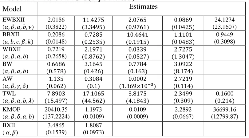
Table 3: MLEs and their SEs (in parentheses)
In Table 2, we compare the fits of the EWBXII distribution with the BBXII, WBXII, BW, AW, TWL, KMOF and BXII distributions. One can see, from Table 1, that the EWBXII distribution has the lowest values for goodness-of-fit statistics among all fitted models. So it could be chosen as the best model for the nicotine data.
The histogram and the estimated densities for nicotine data are displayed in Figure 3. These plots reveal that the EWBXII distribution is the best model to fit this data set. The fitted PDF, CDF, survival function (SF) and Q-Q plots of the EWBXII distribution are shown in Figure 4.
Model Estimates
EWBXII (𝛼, 𝛽, 𝑎, 𝑏, 𝜈) 2.0186 (0.3822) 11.4275 (3.3495) 2.0765 (0.9761) 0.0869 (0.0425) 24.1274 (23.1607) BBXII (𝑎, 𝑏, 𝑐, 𝛽, 𝑘) 0.2086 (0.0148) 0.7285 (0.2535) 10.4641 (0.1915) 1.1101 (0.0483) 0.9449 (0.3098) WBXII (𝛼, 𝛽, 𝑎, 𝑏) 0.7219 (0.2658) 2.1971 (0.8762) 0.0339 (0.0527) 2.7275 (1.3047) BW (𝛼, 𝛽, 𝑎, 𝑏) 0.6686 (0.578) 3.1645 (0.426) 0.7784 (0.163) 3.0922 (8.174) AW (𝛼, 𝛽, 𝛾, 𝛿) 1.135 (0.062) 0.3084 (0.1) 0.0002
(1.369×10⁻³) (0.114)2.7219
Figure 4: Fitted PDF of the EWBXII distribution and other fitted PDFs
Figure 5: Fitted PDF, CDF, SFand Q-Q plots of the EWBXII distribution
6. Conclusions
We study a new five-parameter model called the exponentiated Weibull Burr XII (EWBXII) distribution which generalizes the two-parameter Burr XII distribution and …. We provide some mathematical properties of the new family including explicit expansions for the ordinary and incomplete moments, quantile and generating functions and entropies. The maximum likelihood estimation of the model parameters is investigated. By means of a real data application, we show that the EWBXII distribution can provide better fit than some other well-known models.
References
2. Afify, A. Z., Cordeiro, G. M., Ortega, E. M. M., Yousof, H. M. and Butt, N. S. (2017). The four-parameter Burr XII distribution: properties, regression model and applications. Communications in Statistics-Theory and Methods, forthcoming.
3. Afify, A. Z., Nofal, Z. M., Yousof, H. M., El Gebaly, Y. M. and Butt, N. S. (2015). The transmuted Weibull Lomax distribution: properties and application. Pak. J. Stat. Oper. Res., 11, 135-152.
4. Afify, A. Z., Yousof, H. M., Cordeiro, G. M., Nofal, Z. M. and Ahmad, M. (2016). The Kumaraswamy Marshall-Olkin Fréchet distribution with applications. Journal of ISOSS, 2, 41-58.
5. Al-Saiari, A. Y., Baharith, L. A. and Mousa, S. A. (2014). Marshall-Olkin extended Burr type XII distribution. International Journal of Statistics and Probability,3, 78-84. 6. Burr, I. W. (1942). Cumulative frequency functions. Annals of Mathematical
Statistics, 13, 215-232.
7. Cordeiro, G. M., Afify, A. Z., Yousof, H. M., Pescim, R. R. and Aryal, G. R. (2017). The exponentiated Weibull-H family of distributions: theory and applications. Mediterr. J. Math., 14:155.
8. da Silva, R. V., Gomes-Silva, F., Ramos, M. W. A. and Cordeiro, G. M. (2015). The exponentiated Burr XII Poisson distribution with application to lifetime data. International Journal of Statistics and Probability, 4, 112-131.
9. Gomes, A. E., da-Silva, C. Q. and Cordeiro, G. M. (2015). Two extended Burr models: Theory and practice. Communication in Statistics Theory - Methods, 44, 1706-1734.
10.Lee, C., Famoye, F., and Olumolade, O. (2007). Beta-Weibull distribution: some properties and applications to censored data. Journal of modern applied statistical methods, 6, 17.
11.Mead, M. E. (2014). The beta exponentiated Burr XII distribution. Journal of Statistics: Advances in Theory and Applications,12, 53-73
12.Mead, M. E. and Afify, A. Z. (2017). On five parameter Burr XII distribution: properties and applications. South African Statistical Journal, 51, 67 -80.
13.Paranaíba, P. F., Ortega, E. M. M., Cordeiro, G. M. and de Pascoa, M. (2013). The Kumaraswamy Burr XII distribution: theory and practice. Journal of Statistical Computation and Simulation, 83, 2117-2143.
14.Paranaíba, P. F., Ortega, E. M. M., Cordeiro, G. M. and Pescim, R. R. (2011). The beta Burr XII distribution with application to lifetime data. Computation Statistics and Data Analysis, 55, 1118-1136.