On Hybridizations of Fourth Order Kernel of the Beta Polynomial
Family
Siloko Israel Uzuazor
Department of Mathematics and Computer Science, Edo University Iyamho, Nigeria.
siloko.israel@edouniversity.edu.ng, suzuazor@yahoo.com
Ikpotokin Osayomore
Department of Mathematics and Statistics, Ambrose Alli University, Ekpoma, Nigeria. ikpotokinosayomore@yahoo.co.uk
Siloko Edith Akpevwe Department of Statistics,
University of Benin, Benin City, Nigeria. myakpeski@yahoo.com
Abstract
The usual second order nonparametric kernel estimators are of wide uses in data analysis and visualization but constrained with slow convergence rate. Higher order kernels provide a faster convergence rates and are known to be bias reducing kernels. In this paper, we propose a hybrid of the fourth order kernel which is a merger of two successive fourth order kernels and the statistical properties of these hybrid kernels were studied. The results of our simulation with real data example reveals that the proposed hybrid kernels outperformed their corresponding parent’s kernel functions using the asymptotic mean integrated squared error as the criterion function.
Key words: Kernel, Bandwidth, Beta Polynomial, Higher Order Kernel, Asymptotic Mean Integrated Squared Error.
1. Introduction.
One of the very important and fundamental topics in modern statistics is density estimation. Density estimation is the construction of a probability density estimate from a given set of observation. Probability density estimation has wider applications in virtually every field of studies particularly in biological, management, medical, social and pure sciences. There are two basic approaches to density estimation; the parametric and nonparametric approaches. In the parametric approach, a functional form is usually imposed on the density estimate and the required parameters will be the only information needed to be estimated. The functional form and the parameters estimated will produce a parametric density estimator. The maximum likelihood estimators are the commonest parametric estimators with wide ranges of applications. The nonparametric approach allows the set of observations to speak for themselves in determining the unknown distribution without the imposition of a particular distribution. This paper will center on the nonparametric approach with emphasis on one of its methods, the kernel density estimation technique.
tool for analysis and visualization of the distribution of a given data set (Simonoff, 1996; Imaizumi et al., 2018). The univariate kernel density estimator is compactly written as
𝑓̂(x) = 1
𝑛ℎx∑ 𝐾
𝑛
𝑖=1
(x − X𝑖
ℎx ), (1)
where 𝐾(∙) is the kernel function, ℎx is the bandwidth also called the smoothing parameter, X𝑖 are the set of observations and 𝑛 is the sample size. The shape of the resulting estimate is determined by the kernel function while the smoothing applied in the estimation of 𝑓̂(x) is regulated by the bandwidth. The quality of the estimate in Equation (1) is majorly determined by the magnitude of the smoothing parameter, therefore effort has been geared towards an objective choice of the smoothing parameter (Siloko et al., 2018). The kernel function posses the non-negativity property and must satisfy the following conditions
∫ 𝐾(x)𝑑x = 1, ∫ x𝐾(x)𝑑x = 0 and ∫ x2𝐾(x)𝑑x = 𝜇
2(𝐾) ≠ 0 . (2)
The implication of Equation (2) in kernel density estimation is that the kernel function must be a probability density function which must integrate to unity having zero mean and the variance denoted by 𝜇2(𝐾) is greater than zero (Scott, 1992).
The computational simplicity and efficiency of the kernel density estimator with its easy interpretation of results has contributed to the popularity of the method over other nonparametric density estimation methods. Some recent areas of the application of kernel density estimation include image and video processing (Koloda et al., 2013) and estimation of the direction of wind (Hu et al., 2017). In modeling, kernel density estimation is of immerse applications especially in the construction of probability distributions of observations obtained from a system or process (Martinez and Martinez,
2008) and with applications in data streams of very high speed and large volume (Cao et al.,2012).
This paper introduces new hybrid kernels of the classical fourth order kernel of the beta polynomial family with better performance. The remaining part of this article is organized as follows. In Section 2, we briefly discuss higher order kernels and state its asymptotic mean integrated squared error which is the error criterion function. In Section 3, we discuss the beta polynomial kernel family and introduce the higher order kernel with its hybrid using the Jones and Foster (1993) addition construction rule. The simulation results are presented in Section 4 while Section 5 concludes the article.
2. Asymptotic Mean Integrated Squared Error and Higher Order Kernel.
The performance of the kernel estimator in Equation (1) is mainly measured by the asymptotic mean integrated squared error (AMISE). An approximation of Equation (1) using Taylor’s series expansion yields the two components of the AMISE; the integrated variance and the integrated squared bias given by
𝐴𝑀𝐼𝑆𝐸 (𝑓̂(x)) =𝑅(𝐾) 𝑛ℎ +
1
4𝜇2(𝐾)2ℎ4𝑅(𝑓″), (3)
optimal bandwidth that will minimize the AMISE is the solution to the differential equation
𝜕
𝜕ℎ𝐴𝑀𝐼𝑆𝐸(ℎ) =
−𝑅(𝐾)
𝑛ℎ2 + 𝜇2(𝐾)2ℎ3𝑅(𝑓″) = 0.
Therefore, the bandwidth with the minimum AMISE value denoted by ℎAMISE also known as the optimal bandwidth is
ℎAMISE= [ 𝑅(𝐾)
𝜇2(𝐾)2𝑅(𝑓″)] 1 5⁄
× 𝑛−1 5⁄ . (4)
The contribution of the bias component to the asymptotic mean integrated squared error can be carefully reduced by employing higher order kernels. On relaxation of the conditions that every kernel function must satisfy as stated in Equation (2), it will be possible to achieve a better AMISE value in terms of the performance of the kernel. Assuming the order of the kernel function is denoted by 𝑝, on relaxation of the above conditions, we have
∫ 𝐾(x)𝑑x = 1, ∫ x𝑖𝐾(x)𝑑x = 0, 𝑖 = 1,3, … , 𝑝 − 1 and ∫ x𝑝𝐾(x)𝑑x ≠ 0, (5)
where 𝑝 is the order of the kernel. The order of a kernel function 𝑝 is simply the nonzero moment of the kernel and is usually even because all odd moments of symmetric kernels are zero. Non-negative kernel functions are often regarded as second order kernel while higher order kernels usually exhibit negativity over its support interval (Müller, 1988). Generally, a kernel function is of higher order when its order 𝑝 is greater than two, that is , 𝑝 > 2. If the unknown probability density function is continuously differentiable and the kernel 𝐾 is of order 𝑝, then its corresponding AMISE using Taylor’s series expansion is of the form
𝐴𝑀𝐼𝑆𝐸∗(𝑓̂(x)) = 𝑅(𝐾)
𝑛ℎ + 1
(𝑝!)2𝜇𝑝(𝐾)2ℎ2𝑝𝑅(𝑓(𝑝)), (6) where 𝜇𝑝(𝐾)2 is the 𝑝𝑡ℎ moment of the kernel function. The corresponding smoothing parameter that will minimize Equation (6) is of the form
ℎAMISE∗ = [ (𝑝!)2𝑅(𝐾)
2𝑝𝜇𝑝(𝐾)2𝑅(𝑓(𝑝))]
1 (2𝑝+1)⁄
× 𝑛−1 (2𝑝+1)⁄ . (7)
The smoothing parameter from Equation (7) increases with increase in the kernel order which indicates that much benefit is associated with higher order kernel. The smoothing parameter value in Equation (7) will usually result in the smallest value of the asymptotic mean integrated squared error given by (Scott, 1992)
𝐴𝑀𝐼𝑆𝐸∗(𝑓̂(x)) = [𝑅(𝐾)2𝑝𝑅(𝑓(𝑝))
𝜇𝑝(𝐾)−2 ]
1 (2𝑝+1)⁄
× 𝑛−2𝑝 (2𝑝+1)⁄ . (8)
It should be noted that in Equation (7) and Equation (8), the smoothing parameter with the minimum AMISE value is of order 𝑂(𝑛−1 (2𝑝+1)⁄ ) while the AMISE is of order 𝑂(𝑛−2𝑝 (2𝑝+1)⁄ ). Higher order kernels are generally known as bias reducing kernels and their resulting estimates do have negative components.
3. The Beta Polynomial Kernel Functions.
degree of differentiability. The general form of this kernel family for 𝑠 ≥ 0 with {𝑡 ∈
[−1, 1]} is
𝐾[𝑠](𝑡) =
(2𝑠 + 1)!
22𝑠+1(𝑠!)2(1 − 𝑡2)𝑠, (9) where 𝑠 = 0, 1, 2, … , ∞ is the power of the polynomial function (Scott, 1992). It should be known that kernels of this family are supported on the interval [−1, 1]. In this polynomial kernel family, if 𝑠 takes values from 0 to 3, the corresponding kernels will be the Uniform, Epanechnikov, Biweight and Triweight kernels, respectively.
The Uniform kernel is the simplest kernel in this family while the popular Normal kernel is obtained when 𝑠 tends to infinity. The beta polynomial kernels are of great importance especially the Epanechnikov kernel in the computation of the efficiencies of other members of this family. The first four members of this family known as the Epanechnikov, Biweight, Triweight and Quadriweight kernels excluding the Uniform kernel are as follows
𝐾1(𝑡) =
3
4 (1 − 𝑡2). (10) 𝐾2(𝑡) =
15
16 (1 − 𝑡2)2. (11) 𝐾3(𝑡) =
35
32 (1 − 𝑡2)3. (12) 𝐾4(𝑡) =
315
256 (1 − 𝑡2)4. (13)
However, as the value of 𝑠 tends to infinity, the resulting kernel is the popular Gaussian kernel given by
𝐾∅(𝑡) = 1
√2𝜋 𝑒x𝑝 (−
𝑡2
2). (14) The given kernels are second order kernels whose higher order form can be constructed by using either the multiplicative principle of Terrell and Scott (1980) or the additive principle of Jones and Foster (1993). As a result of the slow convergence rate of the second order nonparametric kernel estimators, higher order kernels are usually employed because they can provide a faster convergence rates and are known to be bias reducing kernels (Marron, 1994). In the construction of the higher order forms of the above kernels, we shall employ the additive principle of Jones and Foster (1993) given as
𝐾[𝑝+2](𝑡) =
3
2𝐾[𝑝,𝑠](𝑡) + 1
2𝑡𝐾[𝑝,𝑠]′ (𝑡). (15)
On differentiating Equation (9) with respect to 𝑡, we have
𝐾[𝑠]′ (𝑡) = (2𝑠 + 1)!
22𝑠+1(𝑠!)2𝑠(1 − 𝑡2)𝑠−1(−2𝑡). (16) Substituting Equation (9) and Equation (16) into Equation (15), we have
𝐾[𝑝+2](𝑡) =3 2[
(2𝑠 + 1)!
22𝑠+1(𝑠!)2(1 − 𝑡2)𝑠] +
1 2𝑡 [
(2𝑠 + 1)!
22𝑠+1(𝑠!)2𝑠(1 − 𝑡2)𝑠−1(−2𝑡)]
= 3 2[
(2𝑠 + 1)!
22𝑠+1(𝑠!)2(1 − 𝑡2)𝑠] − 𝑠𝑡2[
(2𝑠 + 1)!
22𝑠+1(𝑠!)2(1 − 𝑡2)𝑠−1]
= ((2𝑠 + 1)!
22𝑠+1(𝑠!)2(1 − 𝑡2)𝑠) [
3 2−
𝑠𝑡2
= ((2𝑠 + 1)!
22𝑠+1(𝑠!)2(1 − 𝑡2)𝑠) [
3(1 − 𝑡2) − 2𝑠𝑡2
2(1 − 𝑡2) ]
= 1 2{(
(2𝑠 + 1)!
22𝑠+1(𝑠!)2(1 − 𝑡2)𝑠−1) {3 − (3 + 2𝑠)𝑡2}}
Hence, the generalised fourth order kernel of the beta polynomial family is of the form
𝐾[4](𝑡) =
1 2{(
(2𝑠 + 1)!
22𝑠+1(𝑠!)2(1 − 𝑡2)𝑠−1) {3 − (3 + 2𝑠)𝑡2} }. (17) The first four members of the fourth order kernel known as the Epanechnikov, Biweight, Triweight and Quadriweight kernels are as follows
𝐾4,1(𝑡) =38 (3 − 5𝑡2). (18)
𝐾4,2(𝑡) =15
32 (3 − 7𝑡2)(1 − 𝑡2). (19) 𝐾4,3(𝑡) =35
64 (3 − 9𝑡2)(1 − 𝑡2)2. (20) 𝐾4,4(𝑡) =315
512 (3 − 11𝑡2)(1 − 𝑡2)3. (21)
Again, as the value of 𝑠 tends to infinity, the resulting fourth order Gaussian kernel is
𝐾4,∅(𝑡) = 1
2√2𝜋 (3 − 𝑡
2)𝑒x𝑝 (− 𝑡2
2). (22)
The negativity of the resulting estimates of higher order kernels implies that they are not probability densities estimates. In ensuring that the resulting estimates of the higher order kernels are probability density estimates and with faster convergence rate, we propose the hybrid kernel of the beta polynomial family.
3.1 The Proposed Fourth Order Hybrid Kernel Functions.
Let 𝑠 + 1 be the immediate next kernel function of the beta polynomial family such that it is the (𝑠 + 1)𝑡ℎ power of Equation (9). Therefore, the required polynomial will take the form
𝐾[𝑠+1](𝑡) =
(2𝑠 + 3)!
22𝑠+3[(𝑠 + 1)!]2(1 − 𝑡2)𝑠+1. (23) On differentiating Equation (23) with respect to 𝑡, we have
𝐾[𝑠+1]′ (𝑡) = (2𝑠 + 3)!
22𝑠+3[(𝑠 + 1)!]2(𝑠 + 1)(1 − 𝑡2)𝑠(−2𝑡). (24) Now, the modified construction rule is of the form
𝐾[𝑝+2](𝑡) =3
2𝐾[𝑝,𝑠+1](𝑡) + 1
2𝑡𝐾[𝑝,𝑠+1]′ (𝑡). (25)
On substituting Equations (23) and (24) into Equation (25) we have
𝐾[𝑝+2](𝑡) =3 2[
(2𝑠 + 3)!
22𝑠+3[(𝑠 + 1)!]2(1 − 𝑡2)𝑠+1]
+1 2𝑡 [
(2𝑠 + 3)!
22𝑠+3[(𝑠 + 1)!]2(𝑠 + 1)(1 − 𝑡2)𝑠(−2𝑡)]
=3 2[
(2𝑠 + 3)!
22𝑠+3[(𝑠 + 1)!]2(1 − 𝑡2)𝑠+1] − 𝑡2(𝑠 + 1) [
(2𝑠 + 3)!
= ((2𝑠 + 3)! (1 − 𝑡
2)𝑠
22𝑠+3[(𝑠 + 1)!]2 ) [
3
2(1 − 𝑡2) − 𝑡2(𝑠 + 1)]
= ((2𝑠 + 3)! (1 − 𝑡2)𝑠 22𝑠+3[(𝑠 + 1)!]2 ) [
3(1 − 𝑡2) − 2𝑡2(𝑠 + 1)
2 ]
= ((2𝑠 + 3)! (1 − 𝑡
2)𝑠
22𝑠+3[(𝑠 + 1)!]2 ) [
3 − {3 + 2(𝑠 + 1)}𝑡2
2 ]
=1 2{(
(2𝑠 + 3)! (1 − 𝑡2)𝑠
22𝑠+3[(𝑠 + 1)!]2 ) [3 − {3 + 2(𝑠 + 1)}𝑡2]} . (26) For any value of 𝑠, Equation (26) will result in the immediate next kernel function of Equation (17). If 𝑠 = 1, the corresponding fourth order kernel is the Biweight kernel given in Equation (19) and when 𝑠 = 2, the resulting kernel is the Triweight kernel given in Equation (20). The proposed hybrid kernel is the resulting kernel from the product of two successive kernel functions of Equation (26) and Equation (17). The hybrid kernel obtained from their merger is of the form
𝐾[4,𝐻𝑦𝑏𝑟𝑖𝑑](𝑡) =12{((2𝑠 + 3)! (1 − 𝑡2)𝑠
22𝑠+3[(𝑠 + 1)!]2 ) [3 − {3 + 2(𝑠 + 1)}𝑡2]}
×1 2{(
(2𝑠 + 1)!
22𝑠+1(𝑠!)2(1 − 𝑡2)𝑠−1) {3 − (3 + 2𝑠)𝑡2} }
=1 2{(
(2𝑠 + 3)(2𝑠 + 2)(2𝑠 + 1)! (1 − 𝑡2)𝑠
22𝑠+122[(𝑠 + 1)]2[(𝑠!)]2 ) [3 − {3 + 2(𝑠 + 1)}𝑡2]}
×1 2{(
(2𝑠 + 1)!
22𝑠+1(𝑠!)2(1 − 𝑡2)𝑠−1) {3 − (3 + 2𝑠)𝑡2} }
= 1 4{(
(2𝑠 + 1)! (1 − 𝑡2)𝑠
22𝑠+1[(𝑠!)]2 ) (
2𝑠 + 3
𝑠 + 1) [3 − {3 + 2(𝑠 + 1)}𝑡2]}
×1 2{(
(2𝑠 + 1)!
22𝑠+1(𝑠!)2(1 − 𝑡2)𝑠−1) {3 − (3 + 2𝑠)𝑡2} }
=1 8{(
(2𝑠 + 1)! (1 − 𝑡2)𝑠
22𝑠+1[(𝑠!)]2 ) 2
(2𝑠 + 3
𝑠 + 1) [3 − {3 + 2(𝑠 + 1)}𝑡2] {
3 − (3 + 2𝑠)𝑡2
(1 − 𝑡2) }}
= 1 8{(
(2𝑠 + 1)! 22𝑠+1[(𝑠!)]2)
2
(1 − 𝑡2)2𝑠−1(2𝑠 + 3
𝑠 + 1) [3 − {3 + 2(𝑠 + 1)}𝑡2][3 − (3 + 2𝑠)𝑡2]}
This can be simply written as
𝐾[4,𝐻𝑦𝑏𝑟𝑖𝑑](𝑡) =1 8(
(2𝑠 + 1)! 22𝑠+1[(𝑠!)]2)
2
(1 − 𝑡2)2𝑠−1𝜶𝜷𝜸 , (27)
where 𝜶 = (2𝑠+3𝑠+1) , 𝜷 = [3 − {3 + 2(𝑠 + 1)}𝑡2] and 𝜸 = {3 − (3 + 2𝑠)𝑡2}. The first four members of the hybrid kernels are as follows
𝐾4,12∗ (𝑡) = 45
256(3 − 7𝑡2)(3 − 5𝑡2)(1 − 𝑡2). (28) 𝐾4,23∗ (𝑡) = 525
𝐾4,34∗ (𝑡) =11025
32768(3 − 11𝑡2)(3 − 9𝑡2)(1 − 𝑡2)5. (30) 𝐾4,45∗ (𝑡) =218295
524288(3 − 13𝑡2)(3 − 11𝑡2)(1 − 𝑡2)7. (31)
The smoothing parameter with the minimum AMISE value of the classical fourth order kernel is 𝑂(𝑛−1 9⁄ ) while the AMISE of the fourth order kernel is 𝑂(𝑛−8 9)⁄ ). However, the smoothing parameter that minimizes the AMISE of the hybrid kernels is 𝑂(𝑛−1 17⁄ ) while the AMISE is 𝑂(𝑛−16 17)⁄ ).
The proposed hybrid kernel is a bias reduction technique from order four to order eight because it involves the product of two fourth order kernels and unlike the classical fourth order kernel, the resulting estimates is a probability density estimate due to absence of negative components. The proposed hybrid kernel is similar to boosting in kernel density estimation introduced by Marzio and Taylor (2005) which involves the multiplication of kernel estimates that resulted in reducing the asymptotic mean integrated squared error.
4. Results and Discussion.
The statistical properties of the proposed hybrid kernels will be considered for the first four members of the family. Also, their performance will be examined using the AMISE as the error criterion function. The first four members of the classical second order kernel of this family are of wide applications because they form the basis when discussing this class of kernels especially the Epanechnikov kernel in terms of optimality with respect to the AMISE. In the investigation of the AMISE of the fourth order kernels and their hybrids, a sample size of one thousand will be used because higher order kernels are only beneficial if the sample size is reasonably large. Also, higher order kernels require larger bandwidth as the order of the kernel increases but with a smaller value of the AMISE. The estimates of the first four members of the beta kernels (i.e. Epanechnikov, Biweight, Triweight and Quadriweight denoted by Ep, Bi, Tr and Qu) of the fourth order kernel and their hybrids are in Figure 1 and Figure 2 respectively. The hybrid kernels produced estimates which are probability densities unlike their parent’s kernels. The statistical properties of the fourth order kernel and their hybrids such as their roughnesses and moments are shown in Table 1 with their AMISE values.
Figure 2: Plots of the first four members of the fourth order hybrid kernels.
First Hybrid Kernel
Second Hybrid Kernel
Third Hybrid Kernel
Fourth Hybrid Kernel
Figure 1: Plots of the fourth order kernels of the Ep, Bi, Tr and Qu.
Epanechnikov Kernel
Biweight Kernel
Triweight Kernel
Quadriweight Kernel
Figure 3: Plots of fourth order Biweight and Triweight with their Hybrid kernel.
Hybrid Kernel
The choice of the Biweight kernel and its immediate neighbour, the Triweight kernel with their hybrid in the illustration of the performance of the hybrid kernel using real data example is due to the fact that in fourth order kernel, the optimal kernel with respect to the asymptotic mean integrated squared error is the Biweight kernel. The optimal kernel with respect to the AMISE in second order kernel is the Epanechnikov kernel while the optimal kernel in the fourth order kernel with respect to the AMISE is the Biweight kernel. As the order of the kernel increases, the optimal kernel with respect to the AMISE also varies (Müller, 1984). Optimality of a kernel function with respect to the AMISE simply means the kernel function with the minimum AMISE value. The kernel estimate of the hybrid kernel in Figure 3 is above the estimates of its parent’s kernel along the waiting time axis implying that there is the tendency for the estimate of its parents to possess a negative component. Again, the estimates of the Biweight and Triweight are similar because they are of the same order.
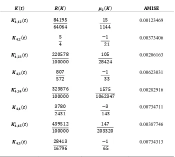
Table 1 shows the classical fourth order kernels of the beta polynomial kernels and their hybrid kernels with their performance using the AMISE. As generally known, one method is better than another when it produces a smaller value of the AMISE (Jarnicka, 2009). The kernel functions denoted by 𝐾∗(𝑡) are the hybrids of the fourth order kernels. The performance of each hybrid kernel is better than the two successive parent’s kernels and this suggests that with large sample sizes, the hybrid kernels of the fourth order kernels will produce better kernel estimates. The results in Table 2 also show that hybrid kernel of the Biweight and Triweight kernels outperformed one of its parents despite the small size of the sample.
𝑲(𝒕) 𝑹(𝑲) 𝝁𝟐(𝑲) 𝐀𝐌𝐈𝐒𝐄
𝑲𝟒,𝟏𝟐∗ (𝒕) 84195
64064
15 1144
0.00123469
𝑲𝟒,𝟐(𝒕) 5
4
−1 21
0.00373406
𝑲𝟒,𝟐𝟑∗ (𝒕) 220578
100000
105 28424
0.00206163
𝑲𝟒,𝟑(𝒕) 807
572
−1 33
0.00623031
𝑲𝟒,𝟑𝟒∗ (𝒕) 323876
100000
1575 1062347
0.00282916
𝑲𝟒,𝟒(𝒕) 3780
2431
−3 143
0.00734711
𝑲𝟒,𝟒𝟓∗ (𝒕) 439512
100000
147 203320
0.00387746
𝑲𝟒,𝟓(𝒕) 28413
16796
−1 65
0.00734313
Higher order kernels are bias reducing kernels resulting in a reduction in the AMISE but associated with the production of estimates with negative components, a situation that requires statistical explanation because the negative components do not improve the AMISE. However, the hybrids of the fourth order kernels as presented in Figure 2 is a probability density estimate with a better performance in terms of the AMISE.
5. Conclusion.
This paper proposed hybrids kernels of the classical fourth order kernels of beta polynomial kernels and investigates their performance using the asymptotic mean integrated squared error as the criterion function. The proposed hybrid kernels are comparable with boosting in kernel density estimation that involves the multiplication of kernel estimates. The results of our simulation and real data example show that the hybrid kernels outperformed the classical fourth order kernels and their estimates are also probability densities.
Acknowledgements.
The authors appreciate the anonymous reviewer and the editorial team for painstakingly going through the manuscript and for their valuable comments and suggestions.
References
1. Azzalini, A. and Bowman, A. W. (1990). A Look at Some Data on the Old Faithful Geyser. Applied Statistics, 39, 357–365.
2. Hu, B., Li, Y., Yang, H. and Wang, H. (2017). Wind Speed Model Based on Kernel Density Estimation and its Application in Reliability Assessment of Generating Systems. Journal of Modern Power Systems and Clean Energy, 5(2), 220–227.
3. Imaizumi, M., Maehara, T. and Yoshida, Y. (2018). Statistically Efficient Estimation for Non-Smooth Probability Densities Proceedings of the 21st International Conference on Artificial Intelligence and Statistics (AISTATS), Lanzarote, Spain. PMLR, 84, 978–987.
4. Jarnicka, J. (2009). Multivariate Kernel Density Estimation with a Parametric Support. Opuscula Mathematica, 29(1), 41–45.
𝑲(𝒕) 𝑹(𝑲) 𝝁𝟐(𝑲) 𝐀𝐌𝐈𝐒𝐄
𝑲𝟒,𝟐(𝒕) 5
4
−1 21
0.0121085
𝑲𝟒,𝟑(𝒕) 807
572
−1 33
0.0192136
𝑲𝟒,𝟐𝟑∗ (𝒕) 220578
100000
105 28424
0.0140592
5. Jones, M. C. and Foster, P. J. (1993). Generalised Jacknifing and Higher Order Kernels. Journal of Nonparametric Statistics, 3, 81–94.
6. Koloda, J., Peinado, A. M. and Sánchez, V. (2013). On the Application of Multivariate Kernel Density Estimation to Image Error Concealment. IEEE International Conference on Acoustics, Speech and Signal Processing, 1330–1334 7. Marron, J. S. (1994). Visual Understanding of Higher-Order Kernels. Journal of
Computational and Graphical Statistics, 3(4), 447–458.
8. Martinez, W. L. and Martinez, A. R. (2008). Computational Statistics Handbook with MATLAB, 2nd ed. London, U.K., Chapman & Hall.
9. Marzio, D. M. and Taylor, C. C. (2005). On Boosting Kernel Density Methods for Multivariate Data: Density Estimation and Classification. Journal of Statistical Methods and Applications, 14, 163–178.
10. Müller, H. G. (1984). Smooth Optimum Estimators of Densities, Regression Curves and Modes. Annals of Statistics, 12, 766–774.
11. M. Müller, H. G. (1988). Nonparametric Regression Analysis of Longitudinal Data. Springer Verlag, Berlin.
12. Scott, D. W. (1992). Multivariate Density Estimation. Theory, Practice and Visualisation. Wiley, New York.
13. Siloko, I. U., Ishiekwene, C. C. and Oyegue, F. O. (2018). New Gradient Methods for Bandwidth Selection in Bivariate Kernel Density Estimation. Mathematics and Statistics, 6(1), 1–8.
14. Simonoff, J. S. (1996). Smoothing Methods in Statistics. Springer-Verlag, New York.