https://doi.org/10.5194/npg-24-581-2017 © Author(s) 2017. This work is distributed under the Creative Commons Attribution 3.0 License.
Balanced source terms for wave generation within
the Hasselmann equation
Vladimir Zakharov1,2,3,4, Donald Resio5, and Andrei Pushkarev1,2,3,4 1Department of Mathematics, University of Arizona, Tucson, AZ 85721, USA 2Lebedev Physical Institute RAS, Leninsky 53, Moscow 119991, Russia 3Novosibirsk State University, Novosibirsk, 630090, Russia
4Waves and Solitons LLC, 1719 W. Marlette Ave., Phoenix, AZ 85015, USA
5Taylor Engineering Research Institute, University of North Florida, Jacksonville, FL, USA
Correspondence to:Andrei Pushkarev ([email protected])
Received: 22 November 2016 – Discussion started: 5 December 2016
Revised: 7 August 2017 – Accepted: 16 August 2017 – Published: 9 October 2017
Abstract.The new Zakharov–Resio–Pushkarev (ZRP) wind input source term (Zakharov et al., 2012) is examined for its theoretical consistency via numerical simulation of the Has-selmann equation. The results are compared to field experi-mental data, collected at different sites around the world, and theoretical predictions based on self-similarity analysis. Con-sistent results are obtained for both limited fetch and duration limited statements.
1 Introduction
The scientific description of wind-driven wave seas, spired by solid state physics statistical ideas (see, for in-stance, Nordheim, 1928), was proposed by Hasselmann (1962, 1963) in the form of the Hasselmann equation (here-after HE), also known as the kinetic equation for waves:
∂ε ∂t +
∂ωk ∂k
∂ε
∂r =Snl+Sin+Sdiss, (1)
where ε=ε(ωk, θ,r, t ) is the wave energy spectrum as a function of wave dispersion ωk=ω(k), angle θ, two-dimensional real space coordinater=(x, y)and timet.Snl,
SinandSdissare the nonlinear, wind input and wave-breaking dissipation source terms, respectively. Hereafter, only the deep water caseω=√gkis considered, wheregis the grav-ity acceleration andk= |k|is the absolute value of the vector wave numberk=(kx, ky).
Since Hasselmann’s work, Eq. (1) has become the basis of operational wave forecasting models such as WAM, SWAN
and Wavewatch III (Tolman, 2013; SWAN, 2015). While the physical oceanography community consents on the general applicability of Eq. (1), there is no consensus on universal parameterizations of the source termsSnl,SinandSdiss. 1.1 TheSnlterm and weak turbulence theory
The HE is a specific example of the kinetic equation for quasi-particles, widely used in different areas of theoreti-cal physics. There are standard methods for its derivation. In the considered case, two forms of theSnlterm were derived by different methods from the Euler equations for free sur-face incompressible potential flow of a liquid by Hasselmann (1962, 1963) and Zakharov and Filonenko (1966). Resio and Perrie (1991) showed that they are identical on the resonant surface:
ωk1+ωk2=ωk3+ωk4, (2)
k1+k2=k3+k4. (3)
The Snl term is the complex nonlinear operator acting on
εk, concealing hidden symmetries (Zakharov and Filonenko, 1967; Zakharov et al., 1992) and cubic with respect to the spectrumε.
To understand the relation and difference between the Boltzmann equation and the HE, one should recall the above-mentioned Nordheim (1928) equation. This equation, appli-cable to quantum quasi-particles, contains both quadratic and cubic terms. Hence, the Boltzmann equation and the HE present opposite limiting cases of a general quantum kinetic equation.
Purely cubical (applicable to classical waves, not to clas-sical particles) systems are relatively new objects in physics. Such equations describe the simplest case of the wave tur-bulence by the theory called weak turtur-bulence theory (WTT) (Zakharov et al., 1992).
It is clear now that the WTT can be used for the de-scription of a very broad class of physical phenomena, in-cluding waves in magneto-hydrodynamics (Galtier et al., 2000), waves in nonlinear optics (Yousefi, 2017), gravita-tional waves in the universe (Galtier and Nazarenko, 2017; de Oliveira et al., 2013), plasma waves (Balk, 2000; Yoon et al., 2016), capillary waves (Pushkarev and Zakharov, 1996; Yulin, 2017; Tran, 2017), and Kelvin waves in super-fluid helium (L’vov and Nazarenko, 2010).
It is unfortunate that the discussion of the HE in the context of WTT has been overlooked by a major part of the oceano-graphic community for many years now. The community ac-cepts, nevertheless, the HE as the basis for the operational wave forecasting models, thereby believing de facto in WTT without fully appreciating its ramifications.
The WTT essentially differs from the kinetic theory of classical particles and quantum quasi-particles. In the “tra-ditional” gas kinetics (both classical and quantum) the ba-sic solutions are thermodynamic equilibrium spectra, such as Boltzmann and Planck distributions. In the WTT such solutions, though formally existing, play no role – they are physical. The physically essential solutions are the non-equilibrium Kolmogorov–Zakharov spectra (or KZ spectra, Zakharov et al., 1992), which are the solutions of the corre-sponding kinetic equation
Snl=0. (4)
The simplest one is the Zakharov–Filonenko (hereafter ZF) solution (Zakharov and Filonenko, 1966), which is the sub-class of KZ solutions:
ε'P 1/3
ω4 , (5)
whereP is the energy flux toward high wave numbers. The accuracy advantage of knowing the analytical expres-sion for theSnlterm, also known in physical oceanography as the XNL, is overshadowed by its computational complexity. Today, none of the operational wave forecasting models can afford to perform XNL computations in real time. Instead, the operational approximation, known as DIA and its deriva-tives, is used to replace this source term. The implication of such simplification is the inclusion of a tuning coefficient
in front of the nonlinear term; however, several publications have shown that DIA does not provide a good approximation of the actual XNL form. The paradigm of replacement of the XNL by DIA and its variations leads to even more grave con-sequences: other source terms must be adjusted to allow the model Eq. (1) to produce desirable results. In other words, deformations suffered by the XNL model due to the replace-ment ofSnlby its surrogates need to be compensated for by non-physical modification of other source terms to achieve reasonable model behavior in any specific case, leading to a loss of physical universality in the HE model.
1.2 Operational formulations for the wind energy input Sinand wave energy dissipationSdissterms
In contrast toSnl, the knowledge ofSinandSdisssource terms is poor; furthermore, both include many heuristic factors and coefficients. The creation of a reliable, well-justified theory ofSinhas been hindered by strong turbulent fluctuations, un-correlated with the wave motions, in the boundary layer over the sea surface. Even one of the most crucial elements of this theory, the vertical distribution of horizontal wind velocity in the region closest to the ocean surface, where wave mo-tions strongly interact with atmospheric momo-tions, is still the subject of debate. The history of the development of differ-ent wind input forms is full of heuristic assumptions, which fundamentally restrict the magnitude and directional distri-bution of this term. As a result, the values of different wind input terms scatter by a factor of 300–500 % (Badulin et al., 2005; Pushkarev and Zakharov, 2016). For example, experi-mental determination ofSin, as provided by direct measure-ments of the momentum flux from the air to the water, cannot be rigorously performed in a laboratory due to gravity wave dispersion dependence on the water depth, as well as prob-lems with scale effects in laboratory winds. Additional infor-mation on the detailed analysis of the current state of the art of wind input terms can be found in Pushkarev and Zakharov (2016).
1.3 Road map for the construction and verification of balanced source terms
The next chapters present a balanced set of wind energy in-put and wave energy dissipation source terms, based on WTT and experimental data analysis. Further, they are numerically checked to comply with WTT predictions and experimental observations. As mentioned above, contrary to previous at-tempts to build the detailed-balance source terms, the current approach is based neither on the development of a rigorous analytic theory of turbulent atmospheric boundary layers nor on reliable and repeatable air to ocean momentum measure-ments. The new Sin is constructed in the artificial way re-alizing, in a sense, “the poor man approach”, based on the finding of a two-parameter family of HE self-similar solu-tions and their restriction to the single-parameter one with the help of comparison with the data of experimental obser-vations, accumulated for several decades.
Section 2 presents experimental evidence of wave energy spectrum characteristics in the form of a specific regression line, found by Resio et al. (2004). The analytic form of this regression line will play a crucial role in narrowing the circle of possible outcomes, obtained with WTT analysis.
Section 3 studies self-similar solutions of the HE – a ki-netic equation for surface ocean waves, starting with the analysis of the behavior of the dissipationless HE in infi-nite space, containing the wind source term in power func-tion form. This approach is similar in spirit to one realized by Zakharov and Filonenko (1967) for finding the solution of the equationSnl=0 in the infinite Fourier domain, which derived the ZF spectrumε∼P1/3
ω4 , whereP is the energy flux toward high wave numbers. The Fourier domain in both sit-uations does not contain any dissipation function: its role is played by infinite phase volume as the effective energy sink at infinitely high wave numbers.
Such a situation is similar to one realized in incompress-ible liquid turbulence for large Reynolds numbers, where the energy distribution is given by the famous Kolmogorov spectrum, transferring the energy from large to small scales, where the energy dissipation is realized due to viscosity, but the viscosity coefficients, i.e., the dissipation details, are not included in the final Kolmogorov spectrum expression. The ZF spectrum and its further KZ generalizations are in this sense the ideological Kolmogorov spectrum counterparts, having the significant difference that the Kolmogorov spec-trum is a plausible conjecture, while KZ spectra are the exact solutions of the wave kinetic equation.
Since the current research is application oriented, it is im-portant to understand why this formally academic approach is connected with reality. In this context, there is no such thing as the dissipation at infinitely small waves in nature: however, it is clear that the existence of an absorption at suf-ficiently high finite frequencies provides a wave scale in real
applications that still preserves the KZ solutions, found from the HE equation in infinite space.
As was mentioned before, this statement was confirmed in a different physical context with radically different inertial ranges (the wave-number band between characteristic energy input and characteristic wave energy dissipation), showing KZ solutions with different corresponding indices. As for the considered case of gravity waves on the surface of a deep fluid, KZ spectra have been routinely observed in multiple experiments. The results, published before 1985, are summa-rized by Phillips (1985). Thereafter, they were observed and discussed by Long and Resio (2007). A complete survey of all measurements requires a separate comprehensive paper, which is in our plans for the future.
The assumed close relation of the HE in the infinite space and finite domain, bounded by high-frequency dissipation, also has a much deeper meaning, consisting in the fact that
Snlis the leading term of the HE (Zakharov, 2010; Zakharov and Badulin, 2011). This allows further use of the solu-tions found from the “zero-dissipation” HE Eq. (13) in in-finite space for “practical” Fourier domains with the dissi-pation localized at finite high enough wave numbers. They take the form of a two-parameter family of self-similar solu-tions, which can be further restricted to the single-parameter one using experimental regression dependence, presented in Sect. 2. These self-similar solutions present realistic HE so-lutions and describe a broad class of wave-energy spectra ob-served in ocean and wave-tank experiments.
The indices, corresponding to self-similar solutions, allow one to wrap up Sect. 3 with the specific form of the wind in-put term in infinite phase space, called the ZRP wind inin-put term (Zakharov et al., 2012; Pushkarev and Zakharov, 2016), with an arbitrary coefficient in front of it. Now, the theoreti-cal part of the wind source termSinconstruction is finished, but the obtained model is not suitable yet for numerical sim-ulation, since to perform in finite phase space, it has to be augmented with the wave-breaking dissipation term.
There is considerable freedom in choosing a specific an-alytic form of such a high-frequency dissipation term, given the lack of a generally accepted rigorous derivation for this mechanism. Consequently, one can choose a preferred one and possibly justify it, but any particular choice will be ques-tioned since it will remain somewhat artificial. Because of that, our motivation was that at the current stage of develop-ment, we considered simplicity as a primary motivating fac-tor. Instead of following the previous path of time-consuming numerical and empirical formulations based on field exper-iments, the authors decided to continue the spectrum from some specific frequency point, well above the spectral peak, with the Phillips law ∼ω−5, which decays faster than the equilibrium spectrumω−4and therefore corresponds to a net wave energy absorption. Although a version of this concept was incorporated by Janssen (2009), detailed forms of this source term have not been developed to date, other than that the spectrum at high frequencies appears to consistently tend toward an ∼ω−5 form as noted by Phillips (1985). Addi-tional evidence for a transition from∼ω−4to∼ω−5at fre-quencies above the equilibrium range comes from analysis of multiple data sets by Resio et al. (2004). In that paper the transition from∼ω−4to∼ω−5occurs approximately at
fd=1.1 Hz; i.e., the physical spectrum has to be continued from this point by∼ω−5.
The spectrum amplitude at the junction frequency fd is dynamically changing in time. It is important that this ana-lytic continuation contributes to a differential in inverse ac-tion, which also affects frequencies lower thanfd, since the nonlinear interaction term Snl is calculated over both “dy-namic” and fixed Phillips areas. Therefore, the Phillips part of the spectrum “sends” the information about the presence of the dissipation abovefdto the rest of the spectrum.
At this point, all that remains for source-term closure in the HE model is the coefficient in front of the wind input term, since it is not well defined experimentally. If we carry out the numerical simulation with some arbitrary chosen coefficient, we could obtain a range of spectral energies but would retain the qualitative properties of the HE, like the∼ω−4spectrum, spectral peak down-shift and peak frequency behavior in ac-cordance with self-similar laws.
To solve this, we choose the wind source coefficient to reproduce the same wave energy growth as was observed in field experiments. The value of this coefficient, found from the comparison with field observations of wave energy growth, is equal to 0.05. This step completes the construction of the HE model.
In the next sections we proceed with numerical simula-tions based on the HE model described above. Section 5 dis-cusses the details of the numerical model setup. Section 6 describes the duration limited numerical simulation, which is the subject of more academic than applied interest, targeted at self-similarity concept support, while the limited fetch nu-merical simulation results, described in Sect. 7, besides aca-demic interest, are the subject of comparison with the field
experiments. A check of the compliance of numerical results with field experimental measurements is presented in Sect. 8.
2 Experimental evidence
Here we examine the empirical evidence from around the world, which has been utilized to quantify energy levels within the equilibrium spectral range by Resio et al. (2004). For convenience, we shall also use the same notation used by Resio et al. (2004) in their study, for the angular av-eraged spectral energy densities in frequency and wave-number spaces:
E4(f )=
2π α4V g
(2πf )4 , (6)
F4(k)=βk−5/2, (7)
wheref = ω
2π,α4is the constant,V is some characteristic velocity andβ=1
2α4V g
−1/2. These notations are based on relation of spectral densities E(f ) and F (k) in frequency
f = ω
2π and wave-numberkbases: F (k)= cg
2πE(f ), (8)
wherecg=ddωk =2·12π g
f is the group velocity.
The notations in Eqs. (6) and (7) are connected with the spectral energy density(ω, θ )through
E(f )=2π
2π Z
0
(ω, θ )dθ. (9)
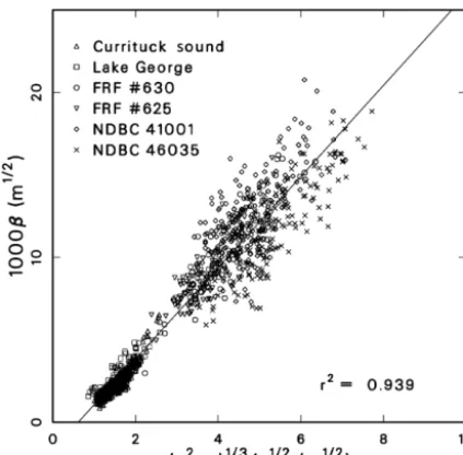
The Resio et al. (2004) analysis showed that experimental en-ergy spectraF (k), estimated through averaginghk5/2F (k)i, can be approximated by a linear regression line as the func-tion of (u2λcp)1/3g−1/2. Figure 1 shows that the regression line
β=1 2α4
h
(u2λcp)1/3−u0
i
g−1/2, (10)
indeed, seems to be a reasonable approximation of these ob-servations.
Here α4=0.00553, u0=1.93 m s−1, cp is the spectral peak phase speed anduλ is the wind speed at the elevation equal to a fixed fractionλ=0.065 of the spectral peak wave-length 2π/kp, where kp is the spectral peak wave number. It is important to emphasize that the Resio et al. (2004) ex-periments show that parameterβincreases with development of the wind-driven sea, whenfpdecreases andCpincreases. This observation is consistent with the weak turbulent theory, whereβ∼P1/3(Zakharov et al., 1992); hereP is the wave energy flux toward small scales.
Resio et al. (2004) assumed that the near-surface bound-ary layer can be treated as neutral and thus follows a conven-tional logarithmic profile
uλ= u∗
κ ln z z0
Figure 1.Correlation of the equilibrium range coefficientβwith
(u2λcp)1/3/g1/2based on data from six disparate sources. Adapted
from Resio et al. (2004).
with a Von Karman coefficientκ=0.41, wherez=λ·2π/kp is the elevation equal to a fixed fraction λ=0.065 of the spectral peak wavelength 2π/kp, where kp is the spectral peak wave number, andz0=αCu2∗/gis subject to Charnock (1955) surface roughness withαC=0.015.
3 Theoretical considerations
Self-similar solutions consistent with the conservative kinetic equation
∂(ω, θ )
∂t =Snl (12)
were studied in Zakharov (2005) and Badulin et al. (2005). In this section we study self-similar solutions of the forced kinetic equation
∂(ω, θ )
∂t =Snl+γ (ω, θ )(ω, θ ) (13)
where(ω, θ )=2ω4
g N (k, θ )is the energy spectrum. One should note that this equation does not contain any ex-plicit wave dissipation term; the role of dissipation is played by the existence of the energy sink at infinitely high wave numbers, in the spirit of the WTT; see Zakharov and Filo-nenko (1967) and Zakharov et al. (1992).
For our purposes, it is sufficient to simply use the dimen-sional estimate forSnl,
Snl'ω
ω5
g2
2
. (14)
Eq. (13) has a self-similar solution if
γ (ω, θ )=αω1+sf (θ ) (15)
wheresis a constant. Looking for a self-similar solution in the form
(ω, t )=tp+qF (ωtq), (16)
we find
q= 1
s+1, (17)
p=9q−1
2 =
8−s
2(s+1). (18)
The functionF (ξ )has a maximum atξ∼ξp; thus, the fre-quency of the spectral peak is
ωp'ξpt−q. (19)
The phase velocity at the spectral peak is
cp=
g ωp
= g ξp
tq= g ξp
ts+11. (20)
According to experimental data, the main energy input into the spectrum occurs in the vicinity of the spectral peak, i.e., at ω'ωp. For ωωp, the spectrum is described by the Zakharov–Filonenko tail
(ω)∼P1/3ω−4. (21)
Here
P = ∞ Z
0 2π Z
0
γ (ω, θ )(ω, θ )dωdθ. (22)
This integral converges ifs <2. For largeω,
(ω, t )'t p−3q
ω4 '
t 2 −s
2(s+1)
ω4 . (23)
More accurately,
(ω, t )'µg ω4u
1−ηcη
pg(θ ), (24)
η=2−s
2 . (25)
Now, supposing s=4/3 and γ'ω7/3, we get η=1/3, which is exactly the experimental regression line prediction. Because it is known from the regression line in Fig. 1 that
ξ=1/3, we immediately get s=4/3 and the wind input term
Swind'ω7/3. (26)
however, Thomson et al. (2013) recently used extensive data from Ocean Station Papa to show that there was minimal wind input into the wave spectrum in the equilibrium range. Resio et al. (2004) suggest that the existence of significant net energy input or dissipation within the frequency range would tend to force the spectrum away from anf−4form, contrary to the pattern found in field measurements. If we as-sume that the wind source is primarily centered on the spec-tral peak, the only missing component in our numerical so-lution is an unknown coefficient in front of it, which will be defined later from the comparison with total energy growth in experimental observations.
Another important theoretical relationship that can be de-rived from joint consideration of Eqs. (6), (8) and (24) is 1000β=λ(u
2c p)1/3
g1/2 , (27)
which shows a theoretical equivalence to the experimental regression, whereλis an unknown constant, defined experi-mentally.
At the end of the section, we present the summary of im-portant relationships.
Wave actionN, energyEand momentumMin frequency-angle presentation are
N = 2
g2 ∞ Z
0 2π Z
0
ω3ndωdφ, (28)
E= 2 g2
∞ Z
0 2π Z
0
ω4ndωdφ, (29)
M= 2
g3 ∞ Z
0 2π Z
0
ω5ncosφdωdφ. (30)
The self-similar relations for the duration limited case are given by
=tp+qF (ωtq), (31)
9q−2p=1, p=10/7, q=3/7, s=4/3, (32)
N ∼tp+q, (33)
E∼tp, (34)
M∼tp−q, (35)
hωi ∼t−q. (36)
The same sort of self-similar analysis gives self-similar re-lations for the fetch limited case:
=χp+qF (ωχq), (37)
10q−2p=1, p=1, q=3/10, s=4/3, (38)
N ∼χp+q, (39)
E∼χp, (40)
M∼χp−q, (41)
hωi ∼χ−q. (42)
4 The details of “implicit” dissipation
Now that the construction of the ZRP wind input term with the unknown coefficient has been accomplished in the spirit of WTT in the previous chapter, the HE model, suitable for numerical simulation, still misses the dissipation term local-ized at finite wave numbers – there is no such thing as the infinite phase volume in reality: the real ocean Fourier space is confined by a characteristic wave number corresponding to the start of the dissipation effects caused by the wave-breaking events.
There is a lot of freedom in choosing the dissipation term. Since there is no current interpretation of the wave-breaking dissipation mechanism, one can choose it in whatever shape it is preferred, but any particular choice will be questioned since it is an artificial one.
Because of that, the motivation consisted in the fact that at the current “proof of concept” stage one needs to know the effective sink with the simplest structure. Continuation of the spectrum fromωdwith the Phillips lawA(ωd)·ω−5(see Phillips, 1966), decaying faster than the equilibrium spec-trum ω−4, will get high-frequency dissipation. The corre-sponding analytic parameterization of this dissipation term will be unknown, while not in principle impossible to figure out in some way. One should note that this method of dissi-pation is not our invention: it is described in Janssen (2009). Specifically, the coefficientA(ωd)in front of ω−5is un-known but is not required to be defined in an explicit form. Instead, it is dynamically determined from the continuity condition of the spectrum, at frequencyωd, on every time step. In other words, the starting point of the Phillips spec-trum coincides with the last point of the dynamically chang-ing spectrum, at the frequency pointωd=2π fd, wherefd' 1.1 Hz, as per Long and Resio (2007). This is the way the high-frequency “implicit” damping is incorporated into the alternative computational framework of the HE. The question of the finer details of the high-frequency “implicit” damping structure is of secondary importance, at the current “proof of concept” stage.
5 Numerical validation of the relationship
To check the self-similar hypothesis posed in Eq. (26), we performed a series of numerical simulations of Eq. (1) in the spatially homogeneous duration limited∂N∂r =0 and spatially inhomogeneous fetch limited ∂N∂t =0 situations.
All simulations used the WRT (Webb–Resio–Tracy) method (see Tracy and Resio, 1982), which calculates the nonlinear interaction term in the exact form. The pre-sented numerical simulation utilized the version of the WRT method, previously used in Webb (1978), Resio and Perrie (1989), Perrie and Zakharov (1999), Pushkarev et al. (2003), Long and Resio (2007), Korotkevich et al. (2008), Zakharov and Badulin (2015), and Pushkarev and Zakharov (2016), and used the grid of 71 logarithmically spaced points in the frequency range from 0.1 to 2.0 Hz and 36 equidistant points in the angle domain. The constant time step in the range be-tween 1 and 2 s has been used for explicit first-order accuracy integration in time.
There is a balance between the number of nodes of the grid and the volume of the calculation to be performed. The par-ticular version of the WRT model has been tuned to the min-imum grid number of nodes to solve realistic physical prob-lems, but is still fast enough to simulate them over a reason-able time span. The correctness of this statement is confirmed by the multiple numerical experiments cited above, repro-ducing mathematical properties of the Hasselmann equation. For convenience, we present the pseudo-code used for the main cycle of the described model.
1. CalculateSnl(ε(f, θ )).
2. Overwriteε(f, θ )tof−5forf >1.1 Hz. 3. Updateε(f, θ )=ε(f, θ )+dt·Snl(f, θ ).
4. Solve analytically ∂(f,θ )∂t =Swind(f, θ )ε(f, θ ) for time dt.
5. Return to step 1.
All numerical simulations discussed in the current paper have been started from a uniform noise energy distribution in Fourier space ε(ω, θ )=10−6m4, corresponding to a small initial wave height with an effectively negligible nonlinearity level. The constant wind of speed 10 m s−1was assumed to blow away from the shoreline, along the fetch. The assump-tion of constant wind speed is a necessary simplificaassump-tion due to the fact that the numerical simulation is being compared to various data from field experiments, and the considered setup is the simplest physical situation which can be modeled.
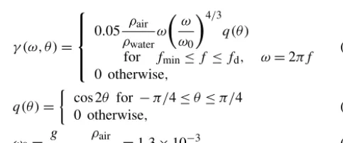
The same ZRP wind input term Eq. (26) has been used in both cases as
Sin(ω, θ )=γ (ω, θ )·ε(ω, θ ), (43)
Duration limited case
0 1•104 2•104 3•104 4•104 tg/U
0.000 0.001 0.002 0.003 0.004
E g
2/U
4
Figure 2.Dimensionless energy Eg2/U4 vs. dimensionless time
tg/Ufor the wind speedU=10 m s−1duration limited case – solid
line. Self-similar solution with the empirical coefficient in front of
it: 1.3×10⁻⁹(tg/U )10/7– dashed line.
γ (ω, θ )=
0.05 ρair
ρwater
ω
ω ω0
4/3 q(θ )
for fmin≤f ≤fd, ω=2πf 0 otherwise,
(44)
q(θ )=
cos 2θ for −π/4≤θ≤π/4
0 otherwise, (45)
ω0=
g U,
ρair
ρwater
=1.3×10⁻³, (46)
whereUis the wind speed at the reference level of 10 m, and
ρairandρwaterare the air and water density, respectively. It is conceivable to use a more sophisticated expression forq(θ ), for instanceq(θ )=q(θ )−q(0). To make direct comparison with experimental results of Resio et al. (2004), we used the relationu∗'U/28 (see Golitsyn, 2010) in Eq. (11). Fre-quenciesfminandfddepend on the wind speed and should be found empirically. In current numerical experiments for
U=10 and U=5 m s−1, fmin=0.1 Hz and fd=1.1 Hz. This choice is justified by the obtained numerical results.
The above-described “implicit dissipation” termSdisshas played the dual role of a direct energy cascade flux sink due to wave breaking as well as a numerical scheme stabilization factor at high wave numbers.
6 Duration limited numerical simulation
The duration limited simulation has been performed for a wind speed ofU=10 m s−1.
Duration limited case
0 1•104 2•104 3•104 4•104 tg/U
0.0 0.5 1.0 1.5 2.0
d ln(E)/d ln(t)
Figure 3.Energy local power function indexp= d lnE
d lnt as a
func-tion of dimensionless timetg/Ufor the wind speedU=10 m s−1
duration limited case – solid line. Theoretical value of the
self-similar indexp=10/7 – thick horizontal dashed line.
Duration limited case
0 1•104 2•104 3•104 4•104 tg/U
0.0 0.2 0.4 0.6 0.8 1.0
<f> U/g
Figure 4.Dimensionless mean frequencyhfi ·U/g=E/N·U/g
(solid line) vs. dimensionless timetg/U for the wind speedU=
10 m s−1 duration limited case – solid line, self-similar solution
with the empirical coefficient in front of it: 16.0·(tg/U )−3/7 –
dashed line.
One should specifically elaborate on the local indexp nu-merical calculation procedure for Fig. 3. First, the total en-ergy function was smoothed via a moving average, then the corresponding derivative is estimated numerically via finite differences, and finally a moving average is used to obtain the time-varying index value.
Duration limited case
0 1•104 2•104 3•104 4•104
tg/U -0.6
-0.5 -0.4 -0.3 -0.2 -0.1 -0.0
d ln(<
>)/d ln(t)
Figure 5.Mean frequency local power function index−q= d lnhωi d lnt
as the function of dimensionless timetg/Ufor the wind speedU=
10 m s−1duration limited case (solid line). Theoretical value of
self-similar exponentq= −3/7 – thick horizontal dashed line.
Duration limited case
0 1•104 2•104 3•104 4•104 tg/U
0.0 0.2 0.4 0.6 0.8 1.0 1.2 1.4
9q-2p
Figure 6.“Magic number” 9q−2pas the function of dimensionless
timetg/Ufor the wind speedU=10 m s−1duration limited case
– solid line. The target value 1 for the self-similar relation Eq. (32) is represented by the horizontal dashed line.
The relatively small systematic deviation from self-similar behavior, visible in Fig. 2, is connected with the following two facts.
Duration limited case
0.1 1.0
f(Hz) 10-5
10-4 10-3 10-2 10-1 100
log(<
>)
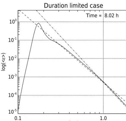
Time = 8.02 h
Figure 7.Decimal logarithm of the angle averaged spectrum as the function of the decimal logarithm of the frequency for the wind
speedU=10 m s−1duration limited case – solid line. Spectrum
∼f−4– dashed line; spectrum∼f−5– dash-dotted line.
take into account the initial transition process. Such a paral-lel shift is equivalent to starting the simulation from different initial conditions.
The second fact is the asymptotic nature of the self-similar solution, producing an evolution of the simulated wave sys-tem toward self-similar behavior with increasing time. As seen in Fig. 3, the numerical value of the local exponent converges to the theoretical value p=10/7, reaching ap-proximately 6 % accuracy for a sufficient dimensionless time 3×10⁴.
The dependence of the mean frequency on time, shown in Fig. 4, is consistent with the self-similar dependence found in Eq. (36) forq=3/7, supplied with the empirical coefficient in front of it: see Fig. 5.
The systematic deviation of two lines in Fig. 4 remains within 3 % of the target valueq=3/7 for the same reasons as for wave-energy behavior – the transition process in the beginning of the simulation and the asymptotic nature of the self-similar solution.
A check of the consistency with the “magic number” 9q−2p=1 (see Eq. 32) is presented in Fig. 6. The reason for systematic deviation from the target value 1 is obviously connected with the reasons for the systematic deviations of
pandq, as the “magic number” is calculated as their linear combination, reaching the accuracy of approximately 10 % for a long enough dimensionless time of 3×10⁴.
One should note that indicesp andq and the “magic re-lation” 9q−2pexhibit asymptotic convergence to the corre-sponding target values.
Duration limited case
0.5 1.0 1.5
f(Hz) 0.000
0.002 0.004 0.006 0.008 0.010 0.012
F(k) k
-5/2
Time = 8.02 h
Figure 8.Compensated spectrum as the function of linear frequency
f for the wind speedU=10 m s−1duration limited case.
Duration limited case
0.5 1.0 1.5
f (Hz) 0
2•10-5 4•10-5 6•10-5 8•10-5 1•10-4
<S
in
> and 0.0001
<
>
Time = 8.02 h
Figure 9. Typical, angle averaged, wind input function density
hSini = 21πRγ (ω, θ )ε(ω, θ )dθ (dotted line) and angle averaged
spectrumhεi = 1
2π R
ε(ω, θ )dθ (solid line) as the functions of the
frequencyf = ω
2π for the wind speedU=10 m s
−1duration
lim-ited case.
Figure 7 presents an angle-integrated energy spectrum as the function of frequency, in logarithmic coordinates. One can see that it consists of the segments of
– the spectral peak region,
– the inertial (equilibrium) rangeω−4spanning from the spectral peak to the beginning of the “implicit dissipa-tion”fd=1.1 Hz, and
-0.4 -0.2 0.0 0.2 0.4 f (Hz)
-0.4 -0.2 0.0 0.2 0.4
f (Hz)
Duration limited case
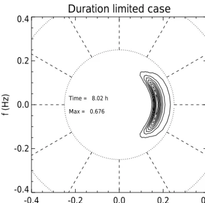
Time = 8.02 h
Max = 0.676
Figure 10.Angular spectrum for the wind speedU=10 m s−1 du-ration limited case.
0 1 2 3 4 5
(U2 C p)
1/3
/g1/2 0
2 4 6 8 10
1000
Figure 11.Experimental, theoretical and numerical evidence of the
dependence of 1000βon(u2λcp)1/3/g1/2. Dashed line –
theoreti-cal prediction Eq. (10) forλ=2.74; dotted line – experimental
re-gression line from Resio et al. (2004) and Long and Resio (2007). Line connected diamonds – results of numerical calculations for the
wind speedU=10 m s−1duration limited case. Being
parameter-ized by dimensionless timetg/U, the numerical simulation
trajec-tory evolves from the left to the right on the graph, covering a time
span fromtg/U=0 totg/U'3.5×105.
The compensated spectrum F (k)·k5/2 is presented in Fig. 8.
One can see a plateau-like region responsible for k−5/2
behavior, equivalent to the∼f−4tail in Fig. 7. This shape of the spectrum is similar to that observed by Long and Re-sio (2007). This exact solution of Eq. (12), known as the KZ spectrum, was found by Zakharov and Filonenko (1967). The
universality off−4asymptotic for the “inertial” (also known as “equilibrium” in oceanography) range between spectral peak energy input and high-frequency energy dissipation ar-eas has been observed in multiple experimental field observa-tions and is accepted by the oceanographic community after the seminal work of Phillips (1985). One should note that most of the energy flux into the system comes in the vicinity of the spectral peak, as shown in Fig. 9, providing a signifi-cant inertial interval for the KZ spectrum.
The angular spectral distribution of energy, presented in Fig. 10, is consistent with the results of experimental obser-vations (Resio et al., 2011) that show a broadening of the angular spreading in both directions away from the spectral peak frequency.
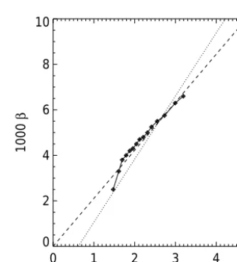
To compare the duration limited numerical simulation re-sults with the experimental analysis by Resio et al. (2004), presented in Fig. 1, Fig. 11 shows the functionβ=F (k)· k5/2as the function of(u2λCp)1/3/g1/2for wind speedU= 10 m s−1, along with the regression line from Resio et al. (2004) and the theoretical prediction Eq. (27) forλ=2.74. The numerical results and theoretical prediction line fall within a very small rms deviation (r2=0.939; see Fig. 1) from the regression line. One should note asymptotic con-vergence of the numerical simulation results to the theoreti-cal line.
7 Limited fetch numerical simulation
The limited fetch simulation was performed in the frame-work of the stationary version of Eq. (1):
1 2
gcosθ ω
∂
∂x=Snl()+Swind+Sdiss, (47)
wherex is chosen as the coordinate axis orthogonal to the shore andθ is the angle between the individual wave num-berk and the axis x. To find the dependence on the wind speed, directed off the shore, two numerical simulations for wind speeds of U=5 m s−1 and U=10 m s−1 have been performed.
The stationarity in Eq. (47) is somewhat difficult for nu-merical simulation, since it contains a singularity in the form of cosθin front of∂x∂. This problem was overcome by zero-ing one-half of the Fourier space of the system for the waves propagating toward the shore. Since the energy in such waves is small with respect to waves propagating in the offshore di-rection, such an approximation is quite reasonable for our purposes.
Since the wind forcing indexs in the fetch limited case is similar to that in the duration limited case, the numerical simulation of Eq. (47) has been performed for the same input functions as in the duration limited case with the same low-level energy noise initial conditions in Fourier space.
Limited fetch case
0 5.0•103
1.0•104
1.5•104
2.0•104
2.5•104
3.0•104
xg/U2
0.000 0.002 0.004 0.006 0.008 0.010
Eg
2/U
2
Figure 12.Dimensionless energyEg2/U4vs. dimensionless fetch
xg/U2for the fetch limited case: wind speedU=10 m s−1– solid
line; wind speedU=5 m s−1– dash-dotted line. Self-similar
solu-tion with the empirical coefficient in front of it: 2.9×10⁻⁷xg/U2
– dashed line.
Limited fetch case
0 5.0•1031.0•104 1.5•104 2.0•1042.5•104 3.0•104
xg/U2 0.0
0.2 0.4 0.6 0.8 1.0 1.2
d ln(E)/d ln(x)
Figure 13. Energy local power function indexp=d lnE
d lnx as the
function of dimensionless fetchxg/U2for the fetch limited case:
wind speed U=10 m s−1 – solid line; wind speedU=5 m s−1
– dash-dotted line. Theoretical value of self-similar indexp=1 –
thick horizontal dashed line.
index p=1, and its appropriate empirical coefficient. The corresponding values of indices p along the fetch are pre-sented in Fig. 13. The small amplitude oscillations observed in the index behavior can be attributed to the finite grid reso-lution used in the simulation.
The wave evolution for the wind speedU=5 m s−1case is expected to be slower than for theU=10 m s−1case due to the weaker nonlinear interaction term. One can see, in-deed, slower asymptotic convergence of the calculated total
Limited fetch case
0 5.0•103 1.0•1041.5•104 2.0•1042.5•104 3.0•104
xg/U2
0.0 0.2 0.4 0.6 0.8 1.0 1.2
<f> U/g
Figure 14. Dimensionless mean frequency as the function of
the dimensionless fetch, calculated ashfi = 1
2π
R
ωndωdθ
R
ndωdθ , where
n(ω, θ )=ε(ω,θ )
ω is the wave action spectrum, for wind speed
10 m s−1(solid line) and 5 m s−1(dashed line). The dash-dotted
line is the self-similar dependence 3.4·(xg
U2)
−0.3with the
empir-ical coefficient in front of it.
energy local power index to the target valuep=1 for the
U=5 m s−1 case compared to theU=10 m s−1case. The deviation of results from theU=10 m s−1 case relative to the target value does not exceed an error of about 5 %, while for theU=5 m s−1case the error does not exceed 20 %. The role of the relatively short (in time) non-self-similar develop-ment of the wave system at the very beginning of the fetch should be noted as well as the factor contributing to the devi-ation from the target value of indexp=1: the wave system obviously needs some time to evolve into a fully self-similar mode.
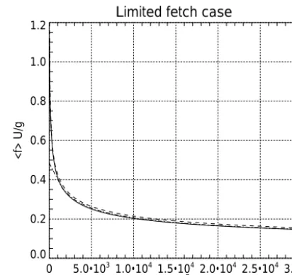
The dependence of the mean frequency on the fetch, shown in Fig. 14, is consistent with the self-similar depen-dence Eq. (42) for indexq=0.3, supplied with the empir-ical coefficient in front of it. The small amplitude oscilla-tions observed in index behavior can be attributed to the finite grid resolution used in the simulation, since the spectral peak moves continuously between discrete frequencies in a man-ner that cannot be matched in these discretized simulations.
The local values of indicesqfor two different wind speed amplitudes are presented in Fig. 15 along with the tar-get value of the self-similar indexq=0.3. After sufficient fetch one can see only about 14 % deviation from the tar-get value for theU=10 m s−1case and about 2.5 % for the
U=5 m s−1case.
Limited fetch case
0 5.0•1031.0•1041.5•1042.0•104 2.5•104 3.0•104
xg/U2
-0.5 -0.4 -0.3 -0.2 -0.1 0.0
d ln(<
>)/d ln(x)
Figure 15. Local mean frequency exponent −q=d lnhωi
d lnx as the
function of dimensionless fetchxg/U2for the limited fetch case.
Wind speedU=10 m s−1– solid line; wind speedU=5 m s−1–
dashed line. Horizontal dashed line – target value of the self-similar
exponentq=0.3.
Limited fetch case
0 5.0•1031.0•104 1.5•1042.0•104 2.5•1043.0•104
xg/U2
0.0 0.5 1.0 1.5 2.0
10q-2p
Figure 16. “Magic number” 10q−2p as a function of
dimen-sionless fetchxg/U2for the limited fetch case. Wind speedU=
10 m s−1– solid line; wind speedU=5 m s−1– dashed line.
Hori-zontal dashed line – self-similar target value 10q−2p=1.
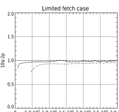
behavior – the transition process in the beginning of the sim-ulation and the asymptotic nature of the self-similar solution. The check on the consistency of the calculated “magic number”(10q−2p)(see Eq. 38) is presented in Fig. 16. The reason for systematic deviation from the target value 1 is ob-viously connected with the systematic deviations ofpandq, as the “magic number” is calculated as their linear combina-tion, reaching the accuracy of approximately 10 % for fetches 3×10⁴. As noted previously, the small amplitude oscillations
Limited fetch case
0.1 1.0
f (Hz) 10-5
10-4 10-3 10-2 10-1
log(<
>)
Fetch = 20.08 km
Figure 17.Decimal logarithm of the angle averaged spectrum as the function of the decimal logarithm of the frequency for the wind
speedU=10 m s−1 limited fetch case – solid line. Spectrum ∼
f−4– dashed line; spectrum∼f−5– dash-dotted line.
Limited fetch case
0.5 1.0 1.5
f (Hz) 0
1•10-5 2•10-5 3•10-5 4•10-5
<S
in
> and 0.0003
<
>
Fetch = 20.08 km
Figure 18.Typical, angle averaged, wind input function density
hSini = 21π R
γ (ω, θ )ε(ω, θ )dθ (dotted line) and angle averaged
spectrumhεi = 1
2π R
ε(ω, θ )dθ (solid line) as the functions of the
frequencyf= ω
2π for the wind speedU=10 m s
−1limited fetch
case.
observed in the indices’ behavior can be attributed to the fi-nite grid resolution used in the simulation.
One should note that indicespandqand the “magic rela-tion” 10q−2pexhibit asymptotic convergence to the corre-sponding target values.
-3 -2 -1 0 1 2 0.00
0.02 0.04 0.06 0.08 0.10 0.12
E/E
tot
Fetch = 20.08 km
Time = 8.02 h
Figure 19. Relative wave energy distribution E(θ )/Etot=
Rfd
fminε(ω, θ )dω/
Rfd fmin
R2π
0 ε(ω, θ )dωdθ as the function of angle θ
for the duration limited (solid line) and limited fetch (dotted line) cases.
Limited fetch case
0.5 1.0 1.5 2.0
f (Hz) 0.000
0.002 0.004 0.006 0.008 0.010 0.012
F(k) k
-5/2
Fetch = 20.08 km
Figure 20. Compensated spectrum as the function of linear
fre-quencyf for the wind speed 10 m s−1limited fetch case.
could be seen in the duration limited case, one can see that it consists of three process-related segments:
– the spectral peak region,
– the inertial (equilibrium) range ω−4spanning from the spectral peak to the beginning of the “implicit dissipa-tion”fd=1.1 Hz, and
– a Phillips high-frequency tail ω−5 starting approxi-mately atfd=1.1 Hz.
The compensated spectrum F (k)·k5/2 is presented in Fig. 20. One can see a plateau-like region responsible for
-0.4 -0.2 0.0 0.2 0.4
f (Hz) -0.4
-0.2 0.0 0.2 0.4
f (Hz)
Limited fetch case
Fetch = 20.08 km
Max = 0.065
Figure 21.Angular spectrum for the wind speedU=10 m s−1 lim-ited fetch case.
0 1 2 3 4 5
(U2 Cp) 1/3
/g1/2 0
2 4 6 8 10
1000
Figure 22.Experimental, theoretical and numerical evidence of the
dependence of 1000βon(u2λcp)1/3/g1/2. Dashed line – theoretical
prediction Eq. (10) forλ=2.11; dotted line – experimental
regres-sion line from Resio et al. (2004) and Long and Resio (2007). Line connected diamonds – the results of numerical calculations for the
wind speedU=10 m s−1limited fetch case. Being parameterized
by the dimensionless fetch coordinateχ= xg
U2, the numerical
sim-ulation trajectory evolves from the left to the right on the graph,
covering a fetch span fromχ=0.toχ'3.0×10⁴.
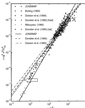
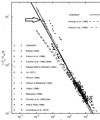
Figure 23. The solid line (pointed to by arrows) presents non-dimensional total energy from the limited fetch numerical experiments, superimposed onto Fig. 5.4, which is adapted from Young (1999). The original caption is “A composite of data from variety of studies showing
the development of the non-dimensional energy,εas a function of non-dimensional fetch,χ. The original JONSWAP study (Hasselmann
et al., 1973) used the data marked, JONSWAP, together with that of Burling (1959) and Mitsuyasu (1968). Also shown are a number of growth curves obtained from the various data sets. These include JONSWAP Eq. (5.27), Donelan et al. (1985) Eq. (5.33) and Dobson et al. (1989) Eq. (5.38).”
between spectral peak energy input and high-frequency en-ergy dissipation areas.
The angular spectral distribution of energy, presented in Fig. 21, as in the duration limited case, is consistent with the results of experimental observations by Resio et al. (2011) that show a broadening of the angular spreading in both di-rections away from the spectral peak frequency.
The excess spectral energy at very oblique angles is a nu-merical artifact connected with the specifics of how the limited fetch statement is simulated here, i.e., the above-mentioned singularity presence on the left-hand side of Eq. (47) atθ= ±π/2.
The detailed structure of angular spreading for both the duration and limited fetch cases is given in Fig. 19. The time that would be required to produce such a pattern is far in excess of the time for this excess energy to be removed from
the equilibrium range by the nonlinear flux and can be shown to vanish when a time–space simulation is used instead of the stationary solution assumed here.
It is clearly seen that the “blobs” in the limited fetch case contain no more than 5 % of the total energy of the corre-sponding spectrum and could be neglected for the purposes of the presented research.
simu-Figure 24.The solid line (pointed to by arrows) presents non-dimensional average frequency as the function of the fetch for limited fetch numerical experiments, superimposed on Fig. 5.5 adapted from Young (1999). The original caption is “A composite of data from a variety
of studies showing the development of the non-dimensional peak frequency, ν as a function of non-dimensional fetch,χ. The original
JONSWAP study (Hasselmann et al., 1973) used all the data shown with the exception of that marked Donelan et al. (1985) and Dobson et al. (1989). Also shown are a number of growth curves obtained from the various data sets. These include JONSWAP Eq. (5.28), Donelan et al. (1985) Eq. (5.34) and Dobson et al. (1989) Eq. (5.39).”
lation results to the theoretical line. Being parameterized by the fetch coordinate, the numerical simulation results evolve from the left to the right on the graph, from the dimensionless fetch equal to 0, to 3.0×10⁴.
8 Comparison with the experiments
A comparison of limited fetch and duration limited simula-tions with the experimental results by Long and Resio (2007) and the theoretical prediction based on Eq. (10) is presented in Figs. 11 and 22. One should note that the numerical results and theoretical prediction line with corresponding values of
λfall into the rms deviation (r2=0.939; see Fig. 1) relative to the experimental regression line Eq. (10).
9 Conclusions
We have analyzed the new ZRP form for wind input, pro-posed in Zakharov et al. (2012) in terms of both fetch limited and duration limited wave growth. The approach proposed here for the development of a set of balanced source terms uses only two empirical coefficients: one in the magnitude of the wind source term and the second in the location of the transition from the∼ω−4to∼ω−5spectrum. This approach focuses on the combination of the theoretical finding of the self-similar solutions and the extraction of the relevant one through the comparison with the field experimental data.
The numerical simulations for both the duration limited and fetch limited cases, using the ZRP wind input term, XNL nonlinear term Snland “implicit” high-frequency dis-sipation, show remarkable consistency with predicted self-similar properties of the HE and with the regression line from field studies, relating energy levels in the equilibrium range to wind speed by Resio et al. (2004) and Long and Resio (2007).
The proposed model is the proof of the concept, providing strong support for simplified assumptions, such as disconti-nuity and the fixed frequency transition point of the source terms. The influence of these effects will be studied, in par-ticular, using a more sophisticated approach by Zakharov and Badulin (2012) in the future.
Although the integral parameters of the model have been verified against the experimental observations, the verifica-tion of the spectral details, such as angular spreading, re-quires additional studies.
Observed oscillations of self-similar indices are inter-preted as the effects of the discreteness of the model, which suggests that a study of the influence of the grid resolution on such oscillations is desirable in future research.
A test of the model invariance with respect to wind speed change from 5 to 10 m s−1has already been performed, but further study of the effects of a wider range of wind speed variation on self-similar properties of the model is desired in the future.
At the moment of submission of the manuscript, the main technical obstacle to effective development of a new gener-ation of physically based HE models was insufficiently fast calculation of the exact nonlinear interaction. The transition to the 2-D case requires a radical increase in the calculation speed. We hope that such improvements will be made in the near future.
The authors hope that this new framework will offer addi-tional guidance for the source terms in operaaddi-tional models.
Acknowledgements. The research presented in Sect. 6 has been ac-complished due to the support of the grant “Wave turbulence: the theory, mathematical modeling and experiment” of the Russian Sci-entific Foundation no. 14-22-00174. The research set forth in Sect. 1 was funded by the program of the presidium of RAS: “Nonlinear
dynamics in mathematical and physical sciences”. The research pre-sented in other chapters was supported by ONR grant N00014-10-1-0991.
The authors gratefully acknowledge the support of these foundations.
Edited by: Victor Shrira
Reviewed by: two anonymous referees
References
Badulin, S., Babanin, A. V., Resio, D. T., and Zakharov, V.: Weakly turbulent laws of wind-wave growth, J. Fluid Mech., 591, 339– 378, 2007.
Zakharov, V. E. and Badulin, S. I: The generalized Phillips’ spectra and new dissipation function for wind-driven seas, arXiv:1212.0963v2 [physics.ao-ph], 1–16, https://arxiv.org/abs/ 1212.0963v2, 2015.
Badulin, S. I., Pushkarev, A. N., Resio, D., and Zakharov, V. E.: Self-similarity of wind-driven seas, Nonlin. Proc. Geoph., 12, 891–945, https://doi.org/10.5194/npg-12-891-2005, 2005. Badulin, S. I., Pushkarev, A. N., Resio, D., and Zakharov, V. E.:
Self-similarity of wind-driven sea, Nonlinear Proc. Geoph., 12, 891–945, 2005.
Balk, A. M.: On the Kolmogorov–Zakharov spectra of weak turbu-lence, Physica D, 139, 137–157, 2000.
Charnock, H.: Wind stress on a water surface, Q. J. Roy. Meteor. Soc., 81, 639–640, 1955.
de Oliveira, H. P., Zayas, L. A. P., and Rodrigues, E. L.:
Kolmogorov–Zakharov spectrum in AdS
gravita-tional collapse, Phys. Rev. Lett., 111, 051101,
https://doi.org/10.1103/PhysRevLett.111.051101, 2013. Dyachenko, A. I., Kachulin, D. I., and Zakharov, V. E.: Evolution of
one-dimensional wind-driven sea spectra, JETP Lett., 102, 577– 581, 2015.
Galtier, S. and Nazarenko, S.: Turbulence of weak gravitational waves in the early universe, 6 pp., available at: https://arxiv.org/ abs/1703.09069v2, last acces: 22 September 2017.
Galtier, S., Nazarenko, S., Newell, A., and Pouquet, A.: A weak turbulence theory for incompressible magnetohydrodynamics, J. Plasma Phys., 63, 447–488, 2000.
Golitsyn, G.: The energy cycle of wind waves on the sea surface, Izv. Atmos. Ocean. Phy., 46, 6–13, 2010.
Hasselmann, K.: On the non-linear energy transfer in a gravity-wave spectrum. Part 1. General theory, J. Fluid Mech., 12, 481–500, 1962.
Hasselmann, K.: On the non-linear energy transfer in a gravity wave spectrum. Part 2. Conservation theorems; wave-particle analogy; irrevesibility, J. Fluid Mech., 15, 273–281, 1963.
Irisov, V. and Voronovich, A.: Numerical Simulation of Wave Breaking, J. Phys. Oceanogr., 41, 346–364, 2011.
Janssen, P.: The Interaction of Ocean Waves and Wind, Cam-bridge monographs on mechanics and applied mathematics, Cambridge U.P., 2009.
Long, C. and Resio, D.: Wind wave spectral observations in Cur-rituck Sound, North Carolina, J. Geophys. Res., 112, C05001, https://doi.org/10.1029/2006JC003835, 2007.
Longuet-Higgins, M. S.: A technique for time-dependent, free-surface flow, Proc. R. Soc. Lon. Ser. A, 371, 441–451, 1980a. Longuet-Higgins, M. S.: On the forming of sharp corners at a free
surface, Proc. R. Soc. Lon. Ser. A, 371, 453–478, 1980b. L’vov, V. S. and Nazarenko, S.: Spectrum of Kelvin-wave turbulence
in superfluids, JETP Lett., 91, 428–434, 2010.
Nordheim, L. W.: On the kinetic method in the new statistics and its application in the electron theory of conductivity, Proc. R. Soc. Lon. Ser. A, 119, 689–698, 1928.
Perrie, W. and Zakharov, V. E.: The equilibrium range cascades of wind-generated waves, Eur. J. Mech. B-Fluid., 18, 365–371, 1999.
Phillips, O. M.: The dynamics of the upper ocean, Cambridge monographs on mechanics and applied mathematics, Cam-bridge U. P., 1966.
Phillips, O. M.: Spectral and statistical properties of the equilibrium range in wind-generated gravity waves, J. Fluid Mech., 156, 505– 531, https://doi.org/10.1017/S0022112085002221, 1985.
Pushkarev, A. and Zakharov, V.: Limited fetch
re-visited: comparison of wind input terms, in
sur-face wave modeling, Ocean Model., 103, 18–37,
https://doi.org/10.1016/j.ocemod.2016.03.005, 2016.
Pushkarev, A., Resio, D., and Zakharov, V.: Weak turbulent ap-proach to the wind-generated gravity sea waves, Physica D, 184, 29–63, 2003.
Pushkarev, A. N. and Zakharov, V. E.: Turbulence of
capillary waves, Phys. Rev. Lett., 76, 3320–3323,
https://doi.org/10.1103/PhysRevLett.76.3320, 1996.
Resio, D. and Perrie, W.: Implications of anf−4equilibrium range
for wind-generated waves, J. Phys. Oceanogr., 19, 193–204, 1989.
Resio, D., Long, C., and Perrie, W.: The role of nonlinear momen-tum fluxes on the evolution of directional wind-wave spectra, J. Phys. Oceanogr., 41, 781–801, 2011.
Resio, D. T. and Perrie, W.: A numerical study of nonlinear energy fluxes due to wave-wave interactions in a wave spectrum. Part I: Methodology and basic results, J. Fluid Mech., 223, 603–629, 1991.
Resio, D. T., Long, C. E., and Vincent, C. L.: Equilibrium-range constant in wind-generated wave spectra, J. Geophys. Res., 109, C01018, https://doi.org/10.1029/2003JC001788, 2004.
SWAN: available at: http://swanmodel.sourceforge.net/, (last ac-cess: 22 September 2017), 2015.
Thomson, J., D’Asaro, E. A., Cronin, M. F., Rogers, W. E., Har-court, R. R., and Shcherbina, A.: Waves and the equilibrium range at Ocean Weather Station P, J. Geophys. Res., 118, 1–12, 2013.
Tolman, H. L.: User Manual and System Documentation of WAVE-WATCH III, Environmental Modeling Center, Marine Modeling and Analysis Branch, 2013.
Tracy, B. and Resio, D.: Theory and calculation of the nonlinear energy transfer between sea waves in deep water, WES report 11, US Army Engineer Waterways Experiment Station, Vicks-burg, MS, 1982.
Tran, M. B.: On a quantum Boltzmann type equation in Zakharov’s wave turbulence theory, available at: https://nttoan81.wordpress. com/, last access: 22 September 2017.
Webb, D. J.: Non-linear transfers between sea waves, Deep-Sea Res., 25, 279–298, 1978.
Yoon, P. H., Ziebell, L. F., Kontar, E. P., and Schlickeiser, R.: Weak turbulence theory for collisional plasmas, Phys. Rev. E, 93, 033203, https://doi.org/10.1103/PhysRevE.93.033203, 2016. Young, I. R.: Wind Generated Ocean Waves, Elsevier, Elsevier Sci-ence Ltd., The Boulevard, Langford Lane Kidlington, Oxford OX5 1GB, UK, 1999.
Yousefi, M. I.: The Kolmogorov–Zakharov model for optical fiber communication, IEEE T. Inform. Theory, 63, 377–391, 2017. Yulin, P.: Understanding of weak turbulence of capillary waves,
available at: http://hdl.handle.net/1721.1/108837, last access: 22 September 2017.
Zakharov, V. E.: Theoretical interpretation of fetch limited wind-drivensea observations, Nonlin. Processes Geophys., 12, 1011– 1020, https://doi.org/10.5194/npg-12-1011-2005, 2005. Zakharov, V. E.: Energy balances in a wind-driven sea, Phys.
Scripta, 2010, T142, http://stacks.iop.org/1402-4896/2010/i= T142/a=014052, 2010.
Zakharov, V. E. and Badulin, S. I.: On energy balance in wind-driven sea, Dokl. Akad. Nauk+, 440, 691–695, 2011.
Zakharov, V. E. and Badulin, S. I.: The generalized Phillips’ spectra and new dissipation function for wind-driven seas, available at: http://arxiv.org/abs/arXiv:1212.0963v2, last access: 22 Septem-ber 2017, 2012.
Zakharov, V. E. and Filonenko, N. N.: The energy spectrum for stochastic oscillation of a fluid’s surface, Dokl. Akad. Nauk, 170, 1992–1995, 1966.
Zakharov, V. E. and Filonenko, N. N.: The energy spectrum for stochastic oscillations of a fluid surface, Sov. Phys. Docl., 11, 881–884, 1967.
Zakharov, V. E., L’vov, V. S., and Falkovich, G.: Kolmogorov Spec-tra of Turbulence I: Wave Turbulence, Springer-Verlag, 1992. Zakharov, V. E., Korotkevich, A. O., and Prokofiev, A. O.: On
dissipation function of ocean waves due to whitecapping, in: American Institute of Physics Conference Series, edited by: Simos, T. E., G.Psihoyios, and Tsitouras, C., vol. 1168, 1229– 1237, 2009.