www.earth-syst-dynam.net/7/917/2016/ doi:10.5194/esd-7-917-2016
© Author(s) 2016. CC Attribution 3.0 License.
The impact of structural error on parameter constraint in
a climate model
Doug McNeall1, Jonny Williams2,4, Ben Booth1, Richard Betts1, Peter Challenor3, Andy Wiltshire1, and
David Sexton1
1Met Office Hadley Centre, FitzRoy Road, Exeter, EX1 3PB, UK
2BRIDGE, School of Geographical Sciences, University of Bristol, Bristol, BS8 1SS, UK 3University of Exeter, North Park Road, Exeter, EX4 4QE, UK
4Now at NIWA, 301 Evans Bay Parade, Hataitai, Wellington 6021, New Zealand
Correspondence to:Doug McNeall ([email protected])
Received: 18 April 2016 – Published in Earth Syst. Dynam. Discuss.: 29 April 2016 Revised: 7 November 2016 – Accepted: 7 November 2016 – Published: 24 November 2016
Abstract. Uncertainty in the simulation of the carbon cycle contributes significantly to uncertainty in the pro-jections of future climate change. We use observations of forest fraction to constrain carbon cycle and land surface input parameters of the global climate model FAMOUS, in the presence of an uncertain structural error. Using an ensemble of climate model runs to build a computationally cheap statistical proxy (emulator) of the climate model, we use history matching to rule out input parameter settings where the corresponding climate model output is judged sufficiently different from observations, even allowing for uncertainty.
Regions of parameter space where FAMOUS best simulates the Amazon forest fraction are incompatible with the regions where FAMOUS best simulates other forests, indicating a structural error in the model. We use the emulator to simulate the forest fraction at the best set of parameters implied by matching the model to the Amazon, Central African, South East Asian, and North American forests in turn. We can find parameters that lead to a realistic forest fraction in the Amazon, but that using the Amazon alone to tune the simulator would result in a significant overestimate of forest fraction in the other forests. Conversely, using the other forests to tune the simulator leads to a larger underestimate of the Amazon forest fraction.
We use sensitivity analysis to find the parameters which have the most impact on simulator output and perform a history-matching exercise using credible estimates for simulator discrepancy and observational uncertainty terms. We are unable to constrain the parameters individually, but we rule out just under half of joint parameter space as being incompatible with forest observations. We discuss the possible sources of the discrepancy in the simulated Amazon, including missing processes in the land surface component and a bias in the climatology of the Amazon.
Copyright statement
The works published in this journal are distributed under the Creative Commons Attribution 3.0 License. This license does not affect the Crown copyright work, which is re-usable under the Open Government Licence (OGL). The Creative Commons Attribution 3.0 License and the OGL are interop-erable and do not conflict with, reduce or limit each other.
©Crown copyright 2016
1 Introduction
value over all others. This uncertainty can be represented, for example, by using a range of values for each of the coef-ficients in an ensemble of simulator1runs.
Choosing parameterisation coefficients is a major research effort encompassing domain specific, statistical and compu-tational literature. Coefficients are tuneable by comparing the simulator with observations of the system, by direct mea-surement or from information from theory. There is a long history of using observations to constrain parameterisation coefficients within general circulation models (GCMs), par-ticularly within atmospheric components. Where this is done in a formal probabilistic setting it can provide probability dis-tributions for the parameters of the simulator; this is known as calibration. Choosing a single best parameter set is tun-ing. History matching rules out parameter settings where simulator output is statistically inconsistent with observa-tions, given uncertainty in those observaobserva-tions, uncertainty in knowledge of the simulator, and a given tolerance of error. A well-calibrated simulator should match the underlying dy-namics of a system better and should produce more accurate and (appropriately) tightly constrained predictions.
1.1 Simulator discrepancy
Simulator discrepancy is the systematic difference between a climate model, or simulator, and the system that is repre-sented by that model. It is also known as model (or simu-lator) bias, model error, or structural error. A “best input” approach typically defines discrepancy as the difference be-tween the modelled system and the simulator when run at an input where output from the simulator conveys all it can about the system (see, e.g., Goldstein and Rougier, 2009). A practical definition from Williamson et al. (2014) is that “a climate model bias [simulator discrepancy] represents a structural error if that bias cannot be removed by changing the parameters without introducing more serious biases to the model”. One of the main aims of the model development process is to efficiently identify important simulator discrep-ancies and correct them, or allow them to be taken into ac-count in analyses – for example, during prediction using the simulator (e.g. Sexton et al., 2011).
Simulator discrepancy might be known ahead of time: per-haps a parameterisation of a process occurring at too high a resolution to simulate has a predictable effect on simula-tor behaviour. Alternatively, the discrepancy might be due to some missing and unknown process in the simulator, or to unknown parameterisation values. This might appear as a bias, only becoming apparent when output from the simula-tor is compared with observations of the real system. In both cases, the modeller must have a strategy for dealing with the
1Throughout the paper we often use simulator in place of
“model”, usually to distinguish an Earth system, climate, or other process model from a statistical model.
discrepancy when using the simulator to make judgements about the system.
Simulator discrepancy is a major challenge during calibra-tion. Kennedy and O’Hagan (2001) introduced a Bayesian framework for the task of the calibration of computationally expensive simulators. They urge the specification of a pri-ori estimates of simulator discrepancy and offer methods to learn about that discrepancy by comparison of the simula-tor and observations. Failure to take simulasimula-tor discrepancy into account in calibration can lead to overconfident and in-accurate estimates of the parameters and, consequently, the predictions of the simulator (e.g. Higdon et al., 2008; Bryn-jarsdóttir and O’Hagan, 2014). Often, there is an indeter-minacy between parameter error and simulator discrepancy; that is, should we choose a different set of parameters as rep-resenting the “best” or should we add a simulator discrep-ancy term? Brynjarsdóttir and O’Hagan (2014) point out that strong prior information is required to distinguish between parameter uncertainty and discrepancy, and that this informa-tion is often lacking. Further, even inadequate (as opposed to outright wrong) specification of a simulator discrepancy can lead to overconfidence and bias in parameters and predic-tions.
1.2 Calibration of land surface components
Parametric uncertainty in the land surface and carbon cycle component of models is expected to represent a large fraction of current uncertainty in future climate projections (Booth et al., 2012, 2013; Huntingford et al., 2009). These com-ponents have been introduced into climate simulators more recently, and have not yet been subject to the depth of sys-tematic evaluation as, for example, atmospheric components. There is much focus, therefore, on identifying parameter sets consistent with observed climate metrics and reducing future land carbon cycle uncertainty by identifying parts of simula-tor parameter space inconsistent with observed properties of the real climate system.
ap-proach is that there is limited understanding of what infor-mation a given observed metric implies about the simulator formulation or parameters, or what this might imply about future projected changes.
1.3 Paper aims and outline
We aim to identify parameter sets of the land surface module of the climate simulator FAMOUS where simulator output and observations of forest fraction are consistent to an ac-ceptable degree. An initial attempt using history matching suggests that FAMOUS is unable to simulate the Amazon forest and other forests simultaneously at any set of parame-ters within the experiment design. We argue that this is due to a fundamental simulator discrepancy, which has implications for constraining the input parameters of FAMOUS. We use a number of techniques to characterise and find the drivers of this structural error, before performing a second history match with an appropriate discrepancy function.
In Sect. 2 we describe the ensemble of a climate simulator, with the emulator and history-matching techniques used to explore simulator discrepancy described in Sects. 2.5 and 2.6 respectively. We perform an initial history-matching exercise in Sect. 3.1. We use the emulator to quantify relationships between the simulated forest fraction and a set of simulator input parameters in a sensitivity analysis in Sect. 3.2. Next, we measure the performance of the ensemble in simulating forest fraction in Sect. 3.3. We see how much input space would be ruled out as implausible in various scenarios of data combination and uncertainty budget in Sect. 3.4 and we learn what each individual observation tells us about input space in Sect. 3.5. In Sect. 3.6, we use the emulator and an implausi-bility measure to find the nominal “best” set of parameters for each forest and then project the consequences of using those parameters on the other forests. Finally, we perform a history-matching exercise with a credible discrepancy func-tion to constrain input parameters in Sect. 3.7. In Sect. 4, we discuss the consequences of our findings for simulators of the Amazon rainforest before offering conclusions in Sect. 5.
2 Data and methods
2.1 The FAMOUS climate simulator
We use a pre-existing ensemble of the climate simulator FAMOUS throughout this study. The Fast Met Office UK Universities Simulator, FAMOUS (Jones et al., 2005; Smith et al., 2008), is a reduced-resolution climate simulator, based on, and tuned to replicate, the climate model HadCM3 (Gor-don et al., 2000; Pope et al., 2000). Computational efficiency is gained primarily through reduced resolution. Atmospheric grid boxes are 4 times the size of HadCM3, and ocean grid boxes are also larger. There are fewer levels in the atmo-sphere (11 compared to 19), and the ocean time step is 12 h compared to 1 h for HadCM3. In the atmosphere, the time
step is 1 h, doubled from HadCM3. The dynamic vegetation component is called TRIFFID and is described in detail in Cox (2001). FAMOUS runs approximately 10 times faster than HadCM3, making it ideal for running large ensembles, or long integrations, with modest supercomputing facilities.
Smith (2012) describes improvements to FAMOUS in sea ice, ozone, hydrological cycle conservation, and upper tro-pospheric dynamics. Williams et al. (2013) describe the in-clusion of the carbon cycle in the simulator via perturbed physics ensembles of terrestrial and ocean parameters, of which the terrestrial ensemble is studied in this paper. Most recently, Williams et al. (2014) give details of inclusion of a scheme to simulate the cycling of oxygen in the ocean and its coupling with the carbon cycle.
The inclusion of vegetation in FAMOUS is documented in Williams et al. (2013), which introduces surface tiling in the newer MOSES2 scheme. Five different vegetation types are simulated: broadleaf and needleleaf trees, C3and C4grasses,
and shrubs, each with a fractional coverage in a grid box. Several surface types represent the absence of vegetation: bare soil, land ice, urbanised land use, and inland water. Williams et al. (2013) describe the optimisation of carbon cy-cle parameters in the terrestrial and ocean domains, validated against observations and reanalysis products, and present cli-matologies using both fixed and dynamic vegetation.
2.2 Known biases in the climate of FAMOUS
FAMOUS shows a Northern Hemisphere-winter surface air temperature cold bias with respect to HadCM3 and also the overestimation of the fractions of needleleaf trees in North America and C3 grassland in the northern part of Eurasia.
The initial version of FAMOUS used the MOSES1 surface exchange scheme and did not explicitly describe the inclu-sion of any vegetation cover, instead using grid box aver-ages of surface quantities such as root depth, surface albedo, and roughness length to describe momentum and water ex-change between the surface and the atmosphere. Biases were already present in climate regimes (Gnanadesikan and Stouf-fer, 2006) relevant for the Amazon rainforest. Smith et al. (2008) noted that “the Amazon region is not wet enough for a fully humid region to exist”.
2.3 The ensemble
Table 1.Land surface input parameters for FAMOUS. PFT: plant functional type; LAI: leaf area index.
Parameter Default Units Description
F0 0.875 Ratio of CO2concentrations inside and outside leaves at zero humidity deficit.
LAI_MIN 3 PFT must achieve this value of LAI before starting to contend with other PFTs for growing area. NL0 0.03 kgN/kgC Top leaf nitrogen concentration. The amount of nitrogen per amount of carbon.
R_GROW 0.250 Growth respiration fraction.
TUPP 36 ◦C Control on variation of photosynthesis with temperature. Q10 2 Control on soil respiration with temperature.
V_CRIT_ALPHA 0.5 Control of photosynthesis with soil moisture.
This design builds upon a previous ensemble run by Gre-goire et al. (2010), and implicitly contains a further parame-ter,β, that indexes into that other ensemble. Theβparameter indexes the top 10 performing simulations with regard to the atmospheric climate. Theβ parameter is uncorrelated with any land surface parameters and the simulator output, so we exclude it from the ensemble design, essentially treating it as a nuisance parameter.
Ranges for the land surface parameters follow those used in the study by Booth et al. (2012) and, as that paper makes clear, were chosen for a number of reasons, not necessarily to represent plausible ranges of their uncertainty. However, we are confident that the parameter ranges are wide enough to span the space which might a priori be considered reason-able.
The ensemble simulates the pre-industrial climate, with ensemble members spun up over a 200-year period to en-sure that the vegetation is in equilibrium with the climate at 290 ppm of CO2. The vegetation dynamics component of the
simulator, TRIFFID, is run in “fast spin-up” mode, for the equivalent of 10 000 years for each decade of climate simula-tion, to allow for the long adjustment time of dynamic vege-tation. The climatology is constructed using the final 30-year period of the ensemble.
2.4 Simulator outputs and observations
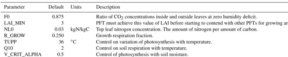
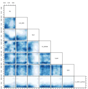
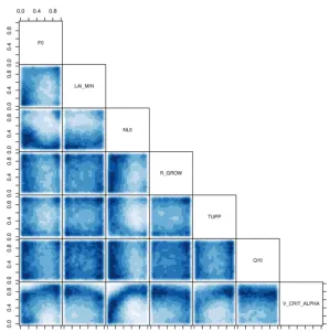
We compare simulated forest fraction against observations adapted from Loveland et al. (2000), consisting of regionally aggregated versions of the data used in the previous study by Williams et al. (2013). We use broadleaf only for the tropi-cal forest, and a mixture of broadleaf and needleleaf for the North American forest. A spatial summary of the ensemble and observations can be found in Fig. 1. Figure 2 shows every input and summary output, plotted against each other. This shows the marginal relationships of the (1) inputs against the inputs (which, as expected, show no obvious relation-ship); (2) the strength of the marginal relationship between the inputs and outputs; and (3) the outputs against the out-puts, which highlights where outputs vary together. Parame-ter ranges do not represent uncertainty, so the ensemble mean and standard deviation are not a meaningful representation of data uncertainty but provide a useful summary of the data. To
summarise the forest fraction data, we find the mean forest fraction in each of the Amazon, Central African, South East Asian, North American, and global regions (see Fig. S1 in the Supplement for region details).
South East Asian and Central African forests vary to-gether very strongly across the ensemble, whereas the Cen-tral African and North American forests show a weaker re-lationship. The latter might be expected, given the different structure of the North American forests, compared with the tropical. The scatter plot also identifies NL0 (leaf nitrogen) and V_CRIT_ALPHA (soil moisture control on photosyn-thesis) as being important controls on forest fraction, as the output seems to vary most with these parameters.
2.5 Training an emulator
FAMOUS is not fast enough to run at every point within in-put space required for our analyses. We therefore use a com-putationally cheap statistical proxy to the simulator, called an emulator. The emulator is a non-parametric regression model conditioned on the ensemble, providing a prediction of sim-ulator output and corresponding uncertainty orders of mag-nitude faster than the original simulator. Once trained, any analysis that might have been done with the simulator can be done with the emulator, provided we include the extra un-certainty term to account for the fact that the emulator is not a perfect prediction of the simulator output. A useful intro-duction to emulators and their uses can be found in O’Hagan (2006), and recent developments in emulator use in climate studies can be found, for example, in Tran et al. (2016) and Bounceur et al. (2015).
0.0 0.2 0.4 0.6 0.8 1.0
Forest fraction
Observations 0.0
0.2 0.4 0.6 0.8 1.0
Forest fraction
Ensemble mean
re
v(lats)
0.00 0.05 0.10 0.15 0.20 0.25 0.30 0.35
Forest fraction
Ensemble standard deviation
Figure 1.Observations of broadleaf forest fraction (top left panel). Mean (top right panel) and standard deviation (bottom left panel) of broadleaf forest fraction across the 100-member ensemble of FAMOUS.
2.6 History matching
After Williamson et al. (2014), we use history matching to find a region of parameter space consistent with observations to within the level of observational and acceptable simulator uncertainty. This requires finding a set of input parameters where the output of the simulator is tolerably close to the ob-servations, given uncertainty in the observations and known deficiencies of the simulator. Constraining parameters in this way helps identify the range of projected futures of the forest consistent with the observations, rather than a single set of “best” parameters.
What distinguishes history matching from simulator cal-ibration, where a probability distribution over the parame-ters is described, is that it rejects inputs inconsistent with observations, or otherwise classifies them as “not ruled out yet” (NROY). We regard NROY inputs as conditionally ac-cepted, contingent on new observations or information. His-tory matching was developed by Craig et al. (1997) and has been used extensively in hydrocarbon extraction sciences and astronomy (e.g. Vernon et al., 2010). Sometimes termed precalibration, it has been used to confront climate simu-lators with observations, for example by Lee et al. (2016), Williamson et al. (2013) and Holden et al. (2009). McNeall et al. (2013) investigated the potential of an observational dataset to constrain input space using history matching.
Observations of the system are denotedz, and we assume that they are made with uncorrelated and independent er-rorssuch thatz=y+, whereyrepresents the true state of
the climate being observed. Denoting the “best” set of input parametersx∗, and assuming the simulator contains a sys-tematic structural errorδ, the observations are related to input parameters
z=g x∗+δ+. (1)
We could find the NROY region forx∗ by running a large number of candidate points of the simulator in a Monte Carlo fashion. FAMOUS is not fast enough for this, and it is also our intention to develop methods that can be used on even more computationally expensive simulators. We therefore use the emulator as a proxy for the simulator output, replac-ingg(x) withη(x) in Eq. (1), and including a term for emu-lator uncertainty in the history-matching calculations.
Each candidate point is assigned an implausibility,I, ac-cording to the emulated forest fraction and uncertainty via Eq. (2). Inputs that produce forest fraction further from the observations are deemed more implausible. Those same in-puts are less implausible if there is greater uncertainty about the observation, the simulator discrepancy, or the emulated output at that input:
I2(x)= |z−E[η(x)]|2/[Var(η(x))+Var(δ)+Var()]. (2)
0.70 0.75 0.80 0.85 0.90 0.95 0.70 0.75 0.80 0.85 0.90 0.95 F0 (INPUT) 1.0 1.5 2.0 2.5 3.0 3.5 4.0 ● ● ● ● ● ● ● ● ● ● ● ● ● ● ● ●●● ● ● ● ●● ● ● ● ● ● ● ● ● ● ● ● ● ● ● ● ● ● ● ● ● ● ● ● ● ● ● ● ● ● ● ●● ● ● ● ● ● ● ● ● ● ● ● ● ● ● ● ● ● ● ● ● ● ● ●● ● ● ● ● ● ● ● ● ● ● ● ● ● ● ● ● ● ● ● ● ● ● LAIMIN (INPUT) 0.02 0.04 0.06 0.08 0.10 ● ● ● ● ● ● ● ● ● ● ● ● ● ● ● ● ● ● ● ● ● ● ● ●● ● ● ● ● ● ● ● ● ● ● ● ● ● ● ● ● ● ● ● ● ● ● ● ● ● ● ● ● ● ● ● ● ● ● ● ● ● ● ● ●● ● ● ● ● ● ● ● ● ● ● ● ● ●● ● ● ● ● ● ● ● ● ● ● ●● ● ● ● ● ● ● ● ● ● ● ● ● ● ● ● ● ● ● ● ● ● ● ● ● ● ● ● ● ● ● ● ● ● ● ● ● ● ● ● ● ● ● ● ● ● ● ● ● ● ● ● ● ● ● ● ● ● ● ● ● ● ● ● ● ● ● ● ● ● ● ● ● ● ● ● ● ● ● ● ● ● ● ● ● ● ● ● ● ● ● ● ● ● ● ● ● ● ● ● ● ●● ● ● ● ● ● ● ● ● NL0 (INPUT) 0.15 0.20 0.25 0.30 0.35 ● ● ● ● ● ● ● ● ● ● ● ● ● ● ● ● ● ● ● ● ● ●● ● ● ● ● ● ● ● ● ● ● ● ● ● ● ● ● ● ● ● ● ● ● ● ● ● ● ● ● ● ● ● ● ● ● ● ● ● ● ● ● ● ● ● ● ● ● ● ● ● ● ● ● ● ● ● ● ● ● ● ● ● ● ● ● ● ● ● ● ● ● ● ● ● ● ● ● ● ● ● ● ● ● ● ● ● ● ● ● ● ● ● ●● ● ● ● ● ● ● ●● ● ● ● ● ● ● ● ● ● ● ● ● ● ● ● ● ● ●● ● ● ● ● ● ● ● ● ● ● ● ● ● ● ● ● ● ● ● ● ● ● ● ● ● ● ● ● ● ● ● ● ● ● ● ● ● ● ● ● ● ● ● ● ● ● ● ● ● ● ● ● ● ● ● ●● ● ● ● ● ● ● ● ● ● ● ● ● ● ● ● ● ● ● ● ● ● ● ● ● ● ● ● ● ● ● ● ● ● ● ● ● ● ● ● ● ● ● ● ● ● ● ● ● ● ● ● ● ● ● ● ● ● ● ● ● ● ● ● ● ● ●● ● ● ● ● ● ● ● ● ● ● ● ● ● ● ● ● ● ● ● ● ● ● ● ● ● ● ● ● ● ● ● ● ● ● ● ● RGROW (INPUT) 32 34 36 38 40 ● ● ● ● ● ● ● ● ● ● ● ● ● ● ● ●● ● ● ● ● ● ● ● ● ● ● ● ● ●● ● ● ● ●● ● ● ● ● ● ● ● ● ●● ● ● ● ● ● ● ● ● ● ● ● ● ● ● ●● ● ● ● ● ● ● ● ●● ● ● ● ● ● ● ● ● ● ● ● ● ● ● ● ● ● ● ● ● ● ● ● ● ● ●●● ● ● ● ● ● ● ● ●● ● ● ● ● ● ● ● ● ●● ● ● ● ● ● ● ● ● ● ● ● ● ● ● ● ● ● ● ●● ● ● ● ● ● ● ● ● ● ● ● ● ● ● ● ● ● ● ● ● ● ● ● ● ● ● ● ● ● ● ● ● ● ● ● ● ● ● ● ● ● ● ● ● ● ● ● ● ● ● ● ● ● ● ● ● ● ● ● ●●● ● ● ● ● ● ●● ● ● ● ● ● ● ● ● ● ● ●● ● ● ● ● ● ● ● ● ● ● ● ● ● ● ● ● ● ● ● ● ●● ● ● ● ● ● ● ● ● ● ● ● ● ● ● ● ● ● ● ● ● ● ● ● ● ● ● ● ● ● ● ● ● ● ● ● ● ● ● ● ● ● ● ● ● ● ● ● ● ● ● ● ● ● ● ● ● ● ●● ● ● ● ● ● ● ● ● ● ● ● ● ● ● ● ● ● ● ● ● ● ● ● ● ● ● ● ● ● ● ● ● ● ● ● ● ● ● ● ● ● ● ● ● ● ● ●● ● ● ● ● ● ● ● ● ● ● ● ● ● ● ● ● ● ● ● ● ● ● ● ● ● ● ● ● ● ● ● ● ● ● ● ● ● ● ● ● ● ● ● ● ● ● ● ● ● ● ● ● ● ● ● ● TUPP (INPUT) 1.5 2.0 2.5 3.0 3.5 ● ● ● ● ● ● ● ● ● ● ● ● ● ● ● ● ● ● ● ● ● ● ● ●● ● ● ● ● ●● ● ● ●● ● ● ● ● ● ● ● ● ● ● ● ● ● ● ● ● ● ● ● ● ● ● ● ● ● ●● ● ● ● ● ● ● ● ● ● ● ● ● ● ● ● ● ● ● ● ● ● ● ● ● ● ● ● ● ● ● ● ● ● ● ● ● ● ● ● ● ● ● ● ● ● ● ● ● ● ● ● ● ●● ● ● ● ● ● ● ● ● ● ● ● ● ● ● ● ● ● ● ● ● ● ● ● ● ● ● ● ● ● ● ● ● ● ● ● ● ● ● ● ● ● ● ● ● ● ● ● ● ● ●●● ● ● ● ● ● ● ● ● ● ● ● ● ● ● ● ● ● ● ● ● ● ● ● ● ● ● ● ● ● ● ● ● ● ● ● ● ● ● ● ● ● ● ● ● ● ● ● ● ● ● ● ● ● ● ● ● ● ● ● ● ● ●● ● ● ● ● ● ● ● ● ● ● ● ● ● ● ● ● ● ● ● ● ● ● ● ● ● ● ● ● ● ● ● ● ● ● ● ●● ● ● ● ● ● ● ● ● ● ● ● ● ● ● ● ● ● ● ● ● ● ● ● ● ● ● ● ● ● ● ● ● ● ● ● ● ● ● ● ● ● ●● ● ● ● ● ● ● ● ● ● ● ● ● ● ● ● ● ● ● ● ● ● ● ● ● ● ● ● ● ● ● ● ● ● ● ● ● ● ● ● ● ● ● ● ● ● ● ● ● ● ● ● ● ● ● ● ● ●● ● ● ● ● ● ● ● ● ● ● ● ● ● ● ● ● ● ● ● ● ● ● ● ● ● ● ● ● ● ● ● ● ● ● ● ● ● ● ● ● ● ● ● ● ● ● ● ● ● ● ● ● ● ● ● ● ● ● ● ● ● ● ● ● ●● ● ● ●● ● ● ● ● ● ● ● ● ● ● ● ● ● ● ● ● ● ● ● ● ● ● ● ● ● ●● ● ● ● ●● ● ● ● ● ● ● ● ● ● ● ● ● ● ● ● ● ● ● ● ● ● ● ● ●● ● ● ● ● ● ● ● ● ● Q10 (INPUT) 0.0 0.2 0.4 0.6 0.8 1.0 ● ● ● ● ● ● ● ● ● ● ● ● ● ● ● ● ● ● ● ● ● ●● ● ● ● ● ● ● ● ● ● ● ● ● ● ● ● ● ● ● ● ● ● ● ● ● ● ● ● ● ● ● ● ● ● ● ● ● ● ● ● ● ● ● ● ● ● ● ●● ● ● ● ● ● ● ●● ● ● ● ● ● ● ● ● ● ● ● ● ● ● ● ● ● ● ● ● ● ● ● ● ● ● ● ● ● ● ● ● ● ● ● ● ● ● ● ● ● ● ●●● ● ● ● ● ● ● ● ● ● ● ● ● ● ● ● ● ● ● ● ● ● ● ● ● ● ● ● ● ● ● ● ● ● ● ● ● ● ● ● ● ● ● ● ● ● ● ● ● ● ● ● ●● ● ● ● ● ● ● ● ● ● ● ● ● ● ● ● ● ● ● ● ● ● ●● ● ● ● ● ● ● ● ● ● ● ● ● ● ● ● ● ● ● ● ● ● ● ● ● ● ● ● ● ● ● ● ● ● ● ● ● ● ● ● ● ● ● ● ● ● ● ● ● ● ● ● ● ● ● ● ● ● ● ● ● ● ● ● ● ● ● ● ● ● ● ● ● ● ● ● ● ● ● ● ● ● ● ● ● ● ● ● ● ● ● ● ● ● ● ● ● ● ● ● ● ● ● ● ● ● ● ● ● ● ●● ● ● ● ● ● ● ● ● ● ● ● ● ● ● ● ● ● ● ● ● ● ● ● ● ● ● ● ● ● ● ● ● ● ● ● ● ● ● ● ● ● ● ● ● ● ● ● ● ● ● ● ● ● ● ● ● ● ● ● ● ● ● ● ● ● ● ● ● ● ● ● ● ● ● ● ● ● ● ● ● ● ● ● ● ● ● ● ● ● ●● ● ● ● ● ● ● ● ● ● ● ● ● ● ● ● ● ● ● ● ● ● ● ● ● ● ● ● ● ● ● ● ● ● ● ● ● ● ● ● ● ● ● ● ● ● ● ● ● ● ● ● ● ● ● ● ● ● ●● ● ● ● ● ● ● ● ● ● ● ●● ●● ● ● ●●● ● ● ● ● ● ● ● ● ● ● ● ● ● ● ● ● ● ● ● ● ● ● ● ● ● ● ● ● ● ● ● ●● ● ● ● ● ● ● ● ● ● ● ● ● ● ● ● ● ● ● ● ● ● ● ● ● ● ● ● ● ● ● ● ● ● ● ● ● ● ● ● ● ● ● ● ● ● ● ● ● ● ● ● ● ● ● ● ● ● ● ● ● ● ● ● ● ● ● ● ● ● ● ● ● ● ● ● ● ● ● ● ● ● ● ● ● ● ●● ● ● ● ● ● ● VCRIT (INPUT) 0.1 0.2 0.3 0.4 0.5 0.6 0.7 ● ● ● ● ● ● ● ● ● ● ●● ● ● ● ●● ● ● ● ● ●● ● ● ● ● ● ●●● ● ● ● ● ● ● ● ● ● ● ● ● ● ● ● ● ● ● ● ● ● ● ● ● ● ● ● ● ● ● ● ● ● ●● ● ● ● ● ● ● ● ● ● ●● ● ● ● ● ● ● ● ● ● ● ● ● ● ● ● ● ● ● ● ● ● ● ● ● ● ● ● ● ● ● ● ● ● ● ● ● ● ● ●● ● ● ● ● ●● ● ● ● ● ● ● ● ●●● ● ● ● ● ● ● ● ● ● ● ● ● ● ● ● ● ● ● ● ● ● ● ● ● ● ● ● ● ● ● ● ● ● ● ● ● ● ● ● ● ● ● ● ● ● ● ● ● ● ● ● ● ● ● ● ● ● ● ●● ● ● ● ● ● ● ● ● ● ● ● ● ● ● ● ● ● ●● ● ● ● ●● ● ● ● ● ● ● ● ● ● ● ● ● ● ●● ● ● ● ● ● ● ●● ● ● ● ● ● ● ● ● ● ● ● ● ● ● ● ● ● ● ● ● ● ● ● ●●● ● ● ● ● ● ● ● ● ● ● ● ● ● ● ● ● ● ● ● ● ● ● ● ● ● ●● ● ● ● ● ● ● ● ● ● ● ● ● ● ● ● ● ● ● ● ● ● ● ● ● ● ● ● ● ● ● ● ● ● ● ● ● ● ● ●● ● ● ● ● ● ●● ● ● ● ● ● ● ● ● ● ● ● ● ● ● ● ● ● ● ● ● ● ● ● ● ●● ● ● ● ● ● ● ● ● ● ● ● ● ● ● ● ● ● ● ● ● ● ● ● ● ● ● ● ● ● ● ● ● ● ● ● ● ● ● ● ● ● ● ● ● ● ● ● ● ● ● ● ● ● ● ● ● ● ● ● ● ● ● ● ●●● ● ● ● ● ● ● ● ● ● ● ● ●● ● ● ● ● ● ● ● ● ● ● ● ● ● ● ● ● ● ● ● ● ● ● ● ● ● ● ● ● ● ● ● ● ● ● ● ● ● ● ● ● ● ● ● ● ● ● ● ● ● ● ● ● ● ● ● ● ● ● ● ● ● ●● ● ● ● ● ● ● ● ● ● ● ● ● ● ● ● ● ● ● ● ● ● ●● ● ● ● ● ● ● ● ● ● ● ● ● ● ● ● ● ● ● ● ● ● ● ● ● ● ● ● ● ● ● ● ● ● ● ● ● ● ● ● ● ● ● ● ● ● ● ● ● ● ● ● ● ● ● ● ● ● ● ● ● ● ● ●● ● ● ● ● ● ● ● ● ● ● ● ● ● ● ● ● ● ● ● ● ●● ● ● ● ● ●● ● ● ● ● ● ● ● ●●● ● ● ● ● ● ● ● ● ● ● ● ● ● ● ● ● ● ● ● ● ● ● ● ● ● ● ● ● ● ● ● ●● ● ● ● ● ● ● ● ● ● ● ● ● ● ● ● ● ● ● ● ● ● ● ● ● ● ● ● ●● ● ● ● ● ● AMAZON (OUTPUT) 0.2 0.4 0.6 0.8 ● ● ● ● ● ● ● ● ● ● ●● ● ● ● ●● ● ● ● ● ● ● ● ● ● ● ● ●●● ● ● ● ● ● ● ● ● ● ● ● ● ● ● ● ● ● ●● ● ● ● ● ● ● ● ● ● ● ● ● ● ● ● ● ● ● ● ● ● ● ● ● ● ● ● ●● ● ● ● ● ● ● ● ● ● ● ● ● ● ● ● ● ● ● ● ● ● ● ● ● ● ● ● ● ● ● ● ● ● ● ● ● ●● ● ● ● ● ● ● ● ● ● ● ● ● ● ●● ● ● ● ● ● ● ● ● ● ● ● ● ● ● ● ● ● ● ● ●● ● ● ● ● ● ● ● ● ● ● ● ● ● ● ● ● ● ● ● ● ● ● ● ● ● ● ● ● ● ● ● ● ● ● ● ● ● ● ●● ● ● ● ● ● ● ● ● ● ● ● ● ● ● ● ● ● ●● ● ● ● ●● ● ● ● ● ● ● ● ● ● ● ● ● ● ● ● ● ● ● ● ● ● ●● ● ● ● ● ● ● ● ● ● ● ●●● ● ● ● ● ● ● ● ● ● ● ●●● ● ● ● ● ● ● ● ● ● ● ● ● ● ● ● ● ● ● ● ● ● ● ● ● ● ●● ● ● ● ● ● ● ● ● ● ● ● ● ● ● ● ● ● ● ● ● ● ● ● ● ● ● ● ● ● ● ● ● ● ● ● ● ● ● ●● ● ● ● ● ● ●● ● ● ● ● ● ● ● ● ●● ● ● ● ● ● ● ● ● ● ● ● ● ● ● ● ● ● ● ● ● ● ● ● ● ● ● ● ● ● ● ● ● ● ● ● ● ● ● ● ● ● ● ● ● ● ● ● ● ● ● ● ● ● ● ● ● ● ● ● ● ● ● ● ● ● ●● ● ● ● ● ● ● ● ● ● ● ● ● ●●● ● ● ● ● ● ● ● ● ● ● ● ●● ● ● ● ● ● ● ● ● ● ● ●● ● ● ● ● ● ● ● ● ● ● ●● ● ● ● ● ● ● ● ● ● ● ● ● ● ● ● ● ● ● ● ● ● ● ● ● ● ● ● ● ● ● ● ● ● ● ● ● ● ● ● ● ● ● ● ● ● ● ● ● ● ● ● ● ● ● ● ● ● ● ● ● ●● ● ● ● ● ● ● ● ● ● ● ● ● ● ● ● ● ● ● ●● ● ● ● ● ● ● ● ● ● ● ● ● ● ● ● ● ● ● ● ● ● ● ● ● ● ● ● ● ● ● ● ● ● ● ● ● ● ● ● ● ● ●●● ● ● ● ● ● ● ● ● ● ● ● ● ● ● ● ● ● ● ● ● ●● ● ● ● ● ● ● ● ● ● ● ● ● ● ● ● ● ● ● ● ● ● ● ● ● ● ● ● ● ● ● ● ●● ●●● ● ● ●● ● ● ● ● ● ● ● ●● ● ●● ● ● ● ● ● ● ● ● ●● ● ● ● ● ● ● ● ● ● ● ● ● ● ● ●● ● ● ● ● ● ● ● ● ● ● ● ● ● ● ● ● ● ● ● ● ● ● ● ● ● ● ● ● ● ● ● ● ● ● ●●● ● ● ● ● ● ● ●● ● ● ● ●● ● ● ● ● ● ●● ● ● ●●● ● ● ● ● ● ● ● ● ● ● ● ● ● ● ● ● ● ● ●● ● ● ● ● ● ● ● ● ● ● ● ● ● ● ●●●● ● ● ● ● ● SEASIA (OUTPUT) 0.2 0.4 0.6 0.8 ● ● ● ● ● ● ● ● ● ● ●● ● ● ● ● ● ● ● ● ● ● ● ● ● ● ● ● ●●● ● ● ● ● ● ● ● ● ● ● ● ● ● ● ● ● ● ● ● ● ● ● ● ● ● ● ● ● ● ● ● ● ● ● ● ● ● ● ● ● ● ● ● ● ●● ● ● ● ● ● ● ● ● ● ● ● ● ● ● ● ● ● ● ● ● ● ● ● ● ● ● ● ● ●● ● ● ●● ● ● ● ● ● ● ● ● ● ●● ● ● ● ● ● ● ● ● ● ●● ● ● ● ● ● ● ● ● ● ● ● ● ● ● ● ● ● ● ●● ● ● ● ● ● ● ● ● ● ● ● ● ● ● ● ● ● ● ● ● ● ●● ● ● ● ● ● ● ● ● ● ● ● ● ● ● ● ●● ● ● ● ● ● ●● ● ● ● ● ● ● ● ● ● ●●● ● ● ● ● ● ● ● ● ● ● ● ● ● ● ● ● ● ● ● ● ● ● ● ● ● ● ● ● ● ● ● ● ● ● ● ● ● ● ●●● ● ● ● ● ● ● ● ● ● ● ●●● ● ● ● ● ● ● ● ● ● ● ● ● ● ● ● ● ● ● ● ● ● ● ● ● ● ●● ● ● ● ● ● ● ● ● ● ● ● ● ● ● ● ● ● ● ● ● ● ● ● ● ● ● ● ● ● ● ● ● ● ● ● ● ● ● ●● ● ● ● ● ● ● ● ● ● ● ● ● ● ● ● ● ● ● ● ● ● ● ● ● ● ● ● ● ● ● ● ● ● ● ● ● ● ● ● ● ● ● ● ● ● ● ● ● ● ● ● ● ● ● ● ● ● ● ● ● ● ● ● ● ● ● ● ● ● ● ● ● ●● ● ● ● ● ● ● ● ● ● ● ● ● ● ● ● ● ● ● ● ● ● ● ●● ● ● ● ● ● ● ● ● ● ● ● ● ● ● ● ● ● ● ● ● ● ● ● ● ●● ● ● ● ● ● ● ● ● ● ● ●● ● ● ● ● ● ● ● ● ● ● ● ● ● ● ● ● ● ● ● ● ● ● ● ● ● ● ● ● ● ● ● ● ● ● ● ● ● ● ● ● ● ● ● ● ● ● ● ● ● ● ● ● ● ● ● ● ● ● ● ● ●● ● ● ● ● ● ● ● ● ● ● ● ●● ● ● ● ● ● ●● ● ● ● ● ● ● ● ● ● ● ● ● ● ● ● ● ● ● ● ● ● ● ● ● ● ● ● ● ● ● ● ● ● ● ● ● ● ● ● ● ● ●●● ● ● ● ● ● ● ● ● ● ● ●● ● ● ●● ● ● ● ● ● ● ● ● ● ●● ● ● ● ● ● ● ● ● ●●● ● ● ● ● ● ● ● ● ● ● ● ● ● ● ● ● ● ● ●● ● ● ●● ● ● ● ● ● ● ● ●● ● ●● ● ● ● ● ● ● ● ● ● ● ● ● ● ● ● ● ● ● ● ● ● ● ● ● ●● ● ● ● ●● ● ● ● ● ● ● ● ● ● ● ● ● ● ● ● ● ● ● ● ● ● ● ● ● ● ● ● ● ● ●● ● ● ● ● ● ● ● ● ● ● ● ● ● ● ● ● ● ● ● ● ● ● ● ●●● ● ● ● ● ● ● ● ● ● ● ● ● ● ● ●● ● ●●● ● ● ● ● ● ● ● ● ● ● ● ● ● ● ●●●● ● ● ● ● ● ● ● ● ● ● ● ● ● ● ● ● ● ● ● ● ● ● ● ● ● ● ● ● ● ● ● ● ● ● ●● ● ● ● ● ● ● ● ● ● ● ● ● ● ● ● ● ● ● ●●●● ● ● ●● ● ● ● ● ● ● ● ● ● ● ● ● ● ● ●● ● ●●● ● ● ● ● ● ● ● ● ● ● ● ● ● ● ●● ●● ● ● ● ● ● CONGO (OUTPUT) 0.1 0.2 0.3 0.4 0.5 ● ● ● ● ● ● ● ● ● ● ● ● ● ● ● ●● ● ● ●● ● ● ● ● ● ● ● ● ●● ● ● ● ● ● ● ● ● ● ● ● ● ● ● ● ● ● ● ● ● ● ● ● ● ● ● ● ● ● ● ● ● ● ● ● ● ● ● ● ● ● ● ● ● ● ● ● ● ● ● ● ● ● ● ● ● ● ● ● ● ● ● ● ● ● ● ● ● ● ● ● ● ● ● ● ● ● ● ● ● ● ● ● ● ●● ● ● ● ●● ● ● ● ● ● ●● ● ●● ● ● ● ● ● ● ● ● ● ● ● ● ● ● ● ● ● ● ● ● ● ● ● ● ● ● ● ● ● ● ● ● ● ● ● ● ● ● ● ● ● ● ● ● ● ● ● ● ● ● ● ● ● ● ● ● ● ● ● ●● ● ● ● ● ● ●● ● ● ● ●● ● ● ● ● ● ● ● ● ● ● ●● ● ● ● ● ● ●● ● ● ● ●● ● ● ● ● ● ● ● ● ● ● ● ● ● ● ● ● ● ● ● ● ● ● ● ● ● ● ● ● ● ● ● ● ● ● ●● ● ● ● ● ● ● ● ● ● ● ● ● ● ● ● ● ● ● ● ● ● ● ● ● ● ●● ● ● ● ● ● ● ● ● ● ● ● ● ● ● ● ● ● ● ● ● ● ● ● ● ● ● ● ●● ● ● ● ● ● ● ● ● ● ● ● ● ● ● ● ● ● ● ● ● ● ● ● ● ● ● ● ● ● ● ● ● ● ● ● ● ● ● ● ● ● ● ● ● ● ● ● ● ● ● ● ● ● ● ● ● ● ● ● ● ● ● ● ● ● ● ● ● ● ● ● ● ● ● ● ● ● ● ● ● ● ● ● ● ● ● ● ● ● ● ● ● ● ● ●● ● ● ● ● ● ● ● ● ● ● ● ● ●●● ● ● ● ● ● ● ● ● ● ● ● ● ● ● ● ● ● ● ● ● ● ● ● ● ● ● ● ● ● ● ● ● ● ● ● ●● ● ● ● ● ●● ● ● ● ● ● ● ● ● ● ● ● ● ● ● ● ●● ● ● ● ● ● ● ● ● ●● ● ● ● ● ● ● ● ● ● ●● ● ● ● ● ● ● ● ● ● ● ● ● ● ● ●● ●● ● ● ● ● ● ● ● ● ● ● ● ●● ● ● ● ● ● ● ● ● ● ● ● ● ● ● ● ● ● ● ● ● ● ● ● ● ● ● ● ● ● ● ● ● ● ● ● ● ● ● ● ● ● ● ● ● ● ● ●● ●● ● ● ● ● ● ● ● ● ● ● ● ● ● ● ● ● ● ● ● ● ● ●● ● ● ● ●● ● ● ● ● ● ●● ● ● ● ● ● ● ● ● ● ● ● ● ● ● ● ● ● ● ● ● ● ● ●● ● ● ● ● ● ● ● ● ● ● ● ● ● ● ●● ● ● ● ● ● ● ● ● ● ● ● ● ● ● ● ● ● ● ● ● ● ● ● ● ● ● ● ● ● ●● ●● ● ● ● ● ● ● ● ● ● ● ● ● ● ● ● ● ● ● ● ● ● ● ● ● ●● ● ●●● ● ● ● ● ● ● ● ● ● ● ● ● ● ● ● ● ● ● ● ● ● ● ● ● ● ● ● ● ● ● ● ● ● ● ● ● ● ● ● ● ● ● ● ● ● ● ● ● ● ● ● ● ● ● ● ● ● ● ● ● ● ● ● ● ● ● ● ● ● ● ● ● ● ● ● ● ● ● ● ● ● ● ● ● ● ● ● ● ● ● ● ● ● ● ● ● ● ●●● ● ● ● ● ● ● ● ● ● ● ● ● ● ● ● ● ● ● ● ● ● ● ● ● ● ● ● ● ● ● ● ● ● ● ● ● ● ● ● ● ● ● ● ● ● ● ● ● ● ● ● ● ● ● ● ● ● ● ●● ● ● ● ● ● ● ● ● ● ● ● ● ● ● ● ● ● ● ● ● ● ● ● ● ● ● ● ● ● ● ● ● ● ● ●●● ●●● ● ● ● ● ● ● ● ● ● ● ● ● ● ● ● ● ● ● ● ● ● ● ● ● ● ● ● ● ● ● ● ● ● ● ● ● ● ● ● ● ● ● ● ● ● ● ● ● ● ● ● ● ● ● ● ● ● ● ●● ● ● ● ● ● ● ● ● NAMERICA (OUTPUT)
0.70 0.75 0.80 0.85 0.90 0.95
0.05 0.10 0.15 0.20 0.25 0.30 ● ● ● ● ● ● ● ● ● ● ●● ● ● ● ● ● ● ● ● ● ● ● ● ● ● ● ● ● ●● ● ● ● ● ● ● ● ● ● ● ● ● ● ● ● ● ● ● ● ● ● ● ● ● ● ● ● ● ● ● ● ● ● ● ● ● ● ● ● ● ● ● ● ● ●● ● ● ● ● ● ● ● ● ● ● ● ● ● ● ● ● ● ● ● ● ● ● ●
1.0 1.5 2.0 2.5 3.0 3.5 4.0 ● ● ● ● ● ● ● ● ● ●● ● ● ● ● ● ● ● ● ● ●● ● ● ● ● ● ● ● ● ●● ● ● ● ● ● ● ● ● ● ● ● ● ● ● ● ● ● ● ● ● ● ● ● ● ● ● ● ● ● ● ● ● ● ● ● ● ● ● ● ● ● ● ●● ● ● ● ● ● ● ● ● ● ● ● ● ● ● ● ● ● ● ● ● ● ● ●●
0.02 0.04 0.06 0.08 0.10 ● ● ● ● ● ● ● ● ● ● ● ● ● ● ● ● ● ● ● ● ● ● ● ● ● ● ● ● ● ● ● ● ● ● ● ● ● ● ● ● ● ● ● ● ● ● ● ● ● ● ● ● ● ● ● ● ● ● ● ● ● ● ● ●● ● ● ● ● ● ● ● ● ● ● ● ● ● ● ● ● ● ● ● ● ● ● ● ● ● ● ● ● ● ● ● ● ● ● ●
0.15 0.20 0.25 0.30 0.35 ● ● ● ● ● ● ● ● ● ● ● ● ● ● ● ● ● ● ● ● ● ● ● ● ● ● ● ● ● ● ● ● ● ● ● ● ● ● ● ● ● ● ● ● ● ● ● ● ● ● ● ● ● ● ● ● ● ● ● ● ● ● ● ● ● ● ● ● ● ● ● ● ● ● ● ● ● ● ● ● ● ● ● ● ● ● ● ● ● ● ● ● ● ● ● ● ● ● ● ●
32 34 36 38 40 ● ● ● ● ● ● ● ● ● ● ● ● ● ● ● ● ● ● ● ● ● ● ● ● ● ● ● ● ● ● ●● ● ● ● ● ● ● ● ● ● ● ● ● ● ● ● ● ● ● ● ● ● ● ● ● ● ● ● ● ● ● ● ● ● ● ● ● ● ● ● ● ● ● ● ● ● ● ● ● ● ● ● ● ● ● ● ● ● ● ● ● ● ● ● ● ● ● ● ●
1.5 2.0 2.5 3.0 3.5 ● ● ● ● ● ● ● ● ● ● ● ● ● ● ● ● ● ● ● ● ● ● ● ● ● ● ● ● ● ●● ● ● ● ● ● ● ● ● ● ● ● ● ● ● ● ● ● ● ● ● ● ● ● ● ● ● ● ● ● ● ● ● ● ● ● ● ● ● ● ● ● ● ● ● ● ● ● ● ● ● ● ● ● ● ● ● ● ● ● ● ● ●● ● ● ● ● ● ●
0.0 0.2 0.4 0.6 0.8 1.0 ● ● ● ● ● ●● ● ● ●● ● ● ● ● ● ● ● ● ● ●● ● ● ● ● ● ● ● ● ● ● ● ● ● ● ● ● ● ● ● ● ● ● ● ● ● ● ● ● ● ●● ● ● ● ● ● ● ● ● ● ● ● ● ● ● ● ● ● ● ● ● ● ● ● ● ● ● ● ● ● ● ● ● ● ● ● ● ● ● ● ● ● ● ● ● ● ●●
0.1 0.2 0.3 0.4 0.5 0.6 0.7 ● ● ● ● ● ● ● ●● ● ● ● ● ● ● ● ● ● ● ● ● ● ● ● ● ● ● ● ● ●●● ● ● ● ● ● ● ● ● ● ● ● ● ● ● ● ● ● ● ● ● ● ● ● ● ● ● ● ● ● ● ● ● ● ● ● ● ● ● ● ●● ● ●● ● ● ● ● ● ● ● ●● ● ● ● ● ● ● ● ● ● ● ● ● ● ● ●
0.2 0.4 0.6 0.8 ● ● ● ● ● ● ● ● ● ● ● ● ● ● ● ● ● ● ● ● ● ● ● ● ● ● ● ● ● ●●● ● ● ● ● ● ● ● ● ● ● ● ● ● ● ● ● ● ● ● ● ● ● ● ● ● ● ● ● ● ● ● ● ● ● ● ● ● ● ● ●● ● ●●● ● ● ● ● ● ● ● ● ● ● ● ● ● ● ● ● ● ● ● ● ● ● ●
0.2 0.4 0.6 0.8 ● ● ● ● ● ● ● ● ● ● ● ● ● ● ● ● ● ● ● ● ● ● ● ● ● ● ● ● ● ● ●● ● ● ● ● ● ● ● ● ● ● ● ● ● ● ● ● ● ● ● ● ● ● ● ● ● ● ● ● ● ● ● ● ● ● ● ● ● ● ● ●● ● ●●● ● ● ● ● ● ● ● ● ● ● ● ● ● ● ● ● ● ● ● ● ● ● ●
0.1 0.2 0.3 0.4 0.5 ● ● ● ● ● ● ● ● ● ●● ● ● ● ● ● ● ● ● ● ● ● ● ● ● ● ● ● ●●● ● ● ● ● ● ● ● ● ● ● ● ● ● ● ● ● ● ● ● ● ● ● ● ● ● ● ● ● ● ● ● ● ●● ● ● ● ● ● ● ● ● ● ●● ● ● ● ● ● ● ● ● ● ● ● ● ● ● ● ● ● ● ● ● ● ● ●●
0.05 0.10 0.15 0.20 0.25 0.30
0.05 0.10 0.15 0.20 0.25 0.30 GLOBAL (OUTPUT)
Figure 2.FAMOUS input parameters and forest fraction parameters, plotted against each other. Default inputs (not run) are marked in red.
probability mass will be contained within 3 standard devia-tions of the mean (Pukelsheim, 1994). Input parameter sets with an implausibility score below the threshold are desig-nated NROY and retained for further analysis. This does not necessarily mean the input settings aregood, merely that evi-dence from observations is not yet sufficient to rule them out as implausible. Inputs may be ruled out as more observations or simulator runs become available.
3 Analyses and results
3.1 An initial history match
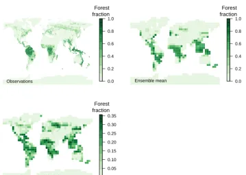
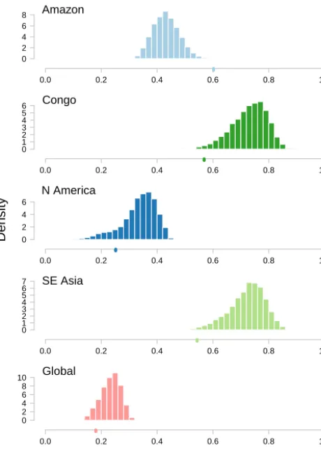
In this section we find regions of land surface parameter space in FAMOUS that remain NROY given some defen-sible assumptions about observational uncertainty. Figure 3 shows how the regionally aggregated simulated forest frac-tion varies across the ensemble, compared with the
corre-sponding observations. Although the simulator was not run with the “standard” parameter settings in the ensemble, we can use the emulator to estimate its output and uncertainty (±1 SD – standard deviation) at those settings; these are shown on the plot, in black.
Amazon
0 5 10 15 20
SE Asia
0 5 10 15 20
Central Africa
0 5 10 15 20
N America
0 5 10 15 20
Global
Mean forest fraction
0.0 0.2 0.4 0.6 0.8 1.0
0 5 10 15 20
● ●
Standard inputs Observation
Figure 3.Histograms representing the number of ensemble mem-bers of a particular forest fraction in each region, as well as globally. Points plotted below the histograms represent the observed forest fraction (colours) and the forest fraction simulated at the “standard” parameters±1 SD (black).
We aim to find regions of parameter space where simula-tor error is removed, or minimised to a level consistent with observational uncertainty. In practice, this requires finding a region where the large negative bias in Amazon forest frac-tion is minimised while keeping the other forests well repre-sented.
On the advice of domain experts, we assume observational uncertainty of 0.05 (1 SD) in the Amazon, Central African, South East Asian, and North American forests as broadly representative, or at least usefully illustrative. This corre-sponds to an expectation that the true 95 % confidence in-terval is contained within the inin-terval of ±0.15, following Pukelsheim’s rule. This is nearly a third of the available range of zero to one, and it would be hard to argue that this repre-sents an over-constraint.
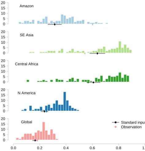
We sample uniformly across input parameter space and run the emulator at these locations. We history-match the samples using all four individual forest observations and vi-sualise the space where max[I]<3. Figure 4 shows a density pairs plot of the approximately 12 % of the 10 000 samples from the emulator that are not ruled out yet by the history match.
Does this region represent a viable set of inputs, perhaps to replace the default set of parameters, or should we include a non-zero discrepancy term (δ in Eq. 1)? Where it appears that we may have found regions where both Amazon and
Table 2.ImplausibilityIof forest observations at default input pa-rameter setting of FAMOUS.
Observation ImplausibilityI
at default parameters
Amazon 3.99
Central Africa 0.56
South East Asia 1.24
North America 0.27
other forests are plausible, we are suspicious of this region, for three reasons. First, the default set of parameters is ruled out, in this case by comparison of the simulator with observa-tions of the Amazon (Table 2). Second, it appears that in the active parameter space projections, these candidates are near the edges and corners of the input space considered plausi-ble. The failure to rule out these points could be due to a relatively large emulator uncertainty, for example. Third, we plot the histograms of the “best estimate” emulator output at these NROY points (Fig. 5), and we see that they can be seen ascompromise candidates. In general, if the simulator is run at points in this region, it will overestimate the Central African, South East Asian, and, most likely, North Ameri-can forest fraction while underestimating the Amazon forest fraction. The candidate points are still included as NROY at these input values because of the combination of the emula-tor uncertainty and the assumed observational uncertainty.
In the remainder of this section, we use a number of anal-ysis techniques to investigate why a region on the edge of pa-rameter space was initially considered plausible, and which does not contain the default parameter settings, is identified as NROY.
3.2 Finding the active parameters with sensitivity analysis
We perform a sensitivity analysis to identify the active sub-space of simulator inputs and quantify relationships between inputs and outputs. In a descriptive sensitivity analysis, we show emulated mean regional and global forest fraction with inputs sampled from across input parameter space in a one-factor-at-a-time fashion, holding all but one parameter at their standard values while varying the remaining parame-ter (Fig. 6). The emulator is not a perfect representation of the simulator, and so we include the emulator uncertainty es-timates at±1 SD, shown as shaded regions in the plot.
0.0 0.4 0.8
0.0
0.4
0.8
F0
0.0
0.4
0.8
LAI_MIN
0.0
0.4
0.8
NL0
0.0
0.4
0.8
R_GROW
0.0
0.4
0.8
TUPP
0.0
0.4
0.8
Q10
0.0 0.4 0.8
0.0
0.4
0.8
0.0 0.4 0.8 0.0 0.4 0.8 0.0 0.4 0.8 0.0 0.4 0.8 0.0 0.4 0.8 0.0 0.4 0.8
0.0
0.4
0.8
V_CRIT_ALPHA
Figure 4.A density pairs plot of two-dimensional projections of parameter space. The blue areas represent the density of NROY points, using all of the data, with an assumed observational uncertainty of 0.05 (1 SD).
Amazon, and not important at all to the North American forests.
The relationships change across parameter space and are therefore dependent on the somewhat arbitrary range of the initial input parameters of the ensemble design. Sensitivity can change in importance as parts of input space are ruled out. For example, the forests are most sensitive to NL0 in the lower part of the ensemble range, and most sensitive to V_CRIT_ALPHA in the upper part of the ensemble range.
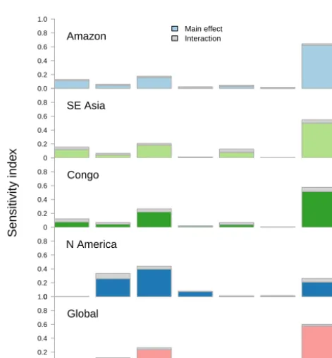
Following Carslaw et al. (2013), we quantify the sensitiv-ity of the simulated forest fraction to the input parameters, using the FAST methodology (Saltelli et al., 1999), conve-niently coded in the R packagesensitivity(Pujol et al., 2015) and easily calculated using the emulator. We calculate the global sensitivity of the simulator output due to each input, as both a main effect and total effect, including interaction terms (Fig. 7). V_CRIT_ALPHA (soil moisture photosyn-thesis control parameter) is the most important parameter across the tropical forests and globally, with a total effect in-dex of around 0.6. In tropical forests, NL0 (leaf nitrogen pa-rameter) is next most important, with a total effect index
be-tween 0.2 and 0.3. In all cases, interaction terms are relatively unimportant, accounting for only a few percent of the vari-ance. North American forests show slightly different results, with NL0 being the most important parameter with a sensi-tivity index near 0.4, followed by LAI_MIN (leaf area index parameter) at around 0.3 and V_CRIT_ALPHA at 0.25. This difference is unsurprising, as the North American forests are a mix of broadleaf and needleleaf trees, which will have dif-ferent sensitivities from a broadleaf tropical forest.
Amazon
0.0 0.2 0.4 0.6 0.8 1.0
0 2 4 6 8
Congo
0.0 0.2 0.4 0.6 0.8 1.0
0 1 2 3 4 5 6
N America
0.0 0.2 0.4 0.6 0.8 1.0
0 2 4 6
SE Asia
0.0 0.2 0.4 0.6 0.8 1.0
0 1 2 3 4 5 6 7
Global
0.0 0.2 0.4 0.6 0.8 1.0
0 2 4 6 8 10
Density
Forest fraction
Figure 5. Best-estimate draws of forest fraction output from the emulator, at the set of points not ruled out yet when assuming a credible observational uncertainty. The value of the observed forest fractions is plotted as a single point on the correspondingxaxes (a “rug plot”).
3.3 Mapping simulator error in parameter space
In this section, we examine the ability of the simulator to reproduce the observed forest fraction, as well as how that ability varies across input parameter space, and assess the region of parameter space which is consistent with each of the forest fraction observations.
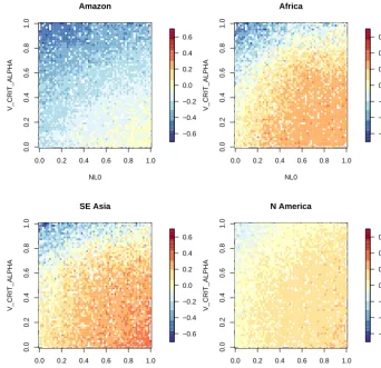
We show a map of simulator error in the two-dimensional space of the most important parameters identified in Sect. 3.2, in Fig. 8. We sample uniformly across all param-eter space, and plot the mean emulated difference between simulator output and the observations for each point. The maps appear noisy because of the impact of randomly cho-sen values of the remaining dimensions, but the structure is clear. For the Central African, South East Asian, and North American forests there is a broad sweep of parameter space, running from low NL0, low V_CRIT_ALPHA to high NL0, high V_CRIT_ALPHA, where simulator error is close to zero. The Amazon input space does not have this region – only the high NL0, high V_CRIT_ALPHA corner has a
sim-ulator error close to zero, suggesting a bias not common to all forests. The lack of overlapping regions where simulator error is close to zero suggests we are unlikely to find a re-gion where we do not need a simulator discrepancy term. It is possible to find a portion of parameter space where the er-ror is similar for all simulator outputs in the low NL0, high V_CRIT_ALPHA corner. However, the error is rather large (at least−0.6) at this point.
3.4 How much input space is ruled out by combinations of observations?
We find the potential of the history-matching technique to rule out parameter space under a number of scenarios of tol-erance to observational and simulator structural error. The denominator of Eq. (2) is the sum of the squared variances of the emulator, discrepancy, and observational uncertainty. Our emulator uncertainty is emergent, but we can experiment by assuming an overall uncertainty budget or by partition-ing assumed uncertainty between observations and simulator discrepancy.
Different observations rule out different parts of param-eter space, while combining observations can be a power-ful method of ruling out large parts of parameter space. A number of approaches to combining data in history matching are discussed in Vernon et al. (2010) and Williamson et al. (2013). A simple strategy is to calculate max[I] at a candi-date input across all data independently and then reject those candidates with a value larger than 3 in any. A danger of this approach is that a single poorly specified emulator or sim-ulator discrepancy term could lead to large swathes of pa-rameter space being incorrectly ruled out. As the number of comparisons with data goes up, so does the probability of including a poorly specified simulator discrepancy. For ex-ample, comparing a simulator with a serious but undiagnosed bias could lead to all a priori plausible parameter space being ruled out as a poor match to the observations. It is important to first combine knowledge and judgement about the system being modelled, and the way that the parameters represent their real-world counterparts (or do not), before relying on observations to remove plausible parameter space.
A conservative approach is to reject a candidate point only if it is judged implausible using a number of measures. This will be more robust to a poorly specified simulator discrep-ancy term. Vernon et al. (2010) use the second and third high-est implausibility score, where a simulator has implausibil-ity scores for multiple outputs calculated. This is to guard against poor emulators, but in practice it works just as well for poorly specified simulator discrepancy. An alternative suggested by Vernon et al. (2010) is to use a multivariate measure of implausibility.
in-F0
0.70 0.75 0.80 0.85 0.90 0.95
0.0 0.2 0.4 0.6 0.8 1.0
F
o
re
s
t fr
a
c
ti
o
n
LAI_MIN
1.0 1.5 2.0 2.5 3.0 3.5 4.0
NL0
0.02 0.04 0.06 0.08 0.10
R_GROW
0.15 0.200.250.300.35
TUPP
32 34 36 38 40
0.0 0.2 0.4 0.6 0.8 1.0
F
orest fr
a
c
ti
o
n
Q10
1.5 2.0 2.5 3.0 3.5
V_CRIT_ALPHA
0.0 0.2 0.4 0.6 0.8 1.0
Amazon Congo Global N America SE Asia
Figure 6.Marginal sensitivity of mean forest fraction to each input parameter in turn, with all other parameters held at standard values. Central lines represent the emulator mean, and shaded areas represent the estimate of emulator uncertainty, at the±1 SD level.
0.0 0.2 0.4 0.6 0.8 1.0
Amazon Main effectInteraction
0 0.2 0.4 0.6
0.8 SE Asia
0 0.2 0.4 0.6
0.8 Congo
0 0.2 0.4 0.6
0.8 N America
F0 LAI_MIN NL0 R_GROW TUPP Q10 V_CRIT_ALPHA 0.0
0.2 0.4 0.6 0.8 1.0
Global
S
e
n
s
it
iv
it
y
in
d
e
x
Figure 7.Sensitivity analysis of forest fraction via the FAST algo-rithm of Saltelli et al. (1999).
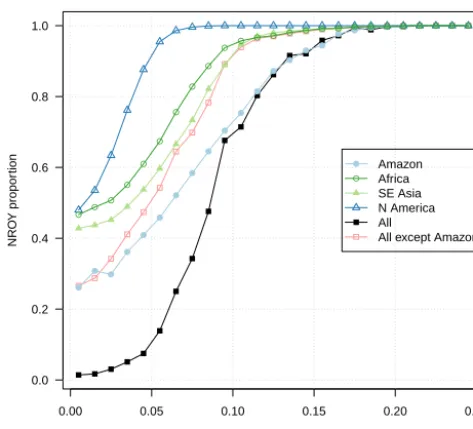
effective for history matching? Figure 9 shows the declining proportion of input parameter space ruled out as we increase tolerance to error in a number of scenarios. Tolerance to error is specified as a single standard deviation, so the full distri-bution of the uncertainty of the observation or discrepancy (e.g. the 95 % range) will be at least 3 times as large, using Pukelsheim’s rule.
North American, South East Asian, and Central African forest observations constrain parameter space to between 40 and 50 % of parameter space, even when our tolerance to error is very low. The proportion of NROY space increases quickly, particularly using North American forest fraction, which becomes no constraint at all when our error tolerance is above 0.07 (1 SD). The other forests offer some constraint up to about 0.1 (1 SD), and the Amazon is more of a con-straint, only losing power as a constraint when the standard deviation of our tolerance to error is above 0.15 (1 SD).
Combining data and using the maximum implausibility of any dataset improves the constraint, particularly when the tolerance to error is low. However, we urge caution. The fact that (a) the performance of the Amazon dataset appears dif-ferent from the other observations and (b) that all parameter space is ruled out at lower values, even though there is emu-lator uncertainty, again raises concerns of a poorly specified Amazon simulator discrepancy.
0.0 0.2 0.4 0.6 0.8 1.0
0.0
0.2
0.4
0.6
0.8
1.0
Amazon
NL0
V_CRIT_ALPHA
−0.6 −0.4 −0.2 0.0 0.2 0.4 0.6
0.0 0.2 0.4 0.6 0.8 1.0
0.0
0.2
0.4
0.6
0.8
1.0
Africa
NL0
V_CRIT_ALPHA
−0.6 −0.4 −0.2 0.0 0.2 0.4 0.6
0.0 0.2 0.4 0.6 0.8 1.0
0.0
0.2
0.4
0.6
0.8
1.0
SE Asia
NL0
V_CRIT_ALPHA
−0.6 −0.4 −0.2 0.0 0.2 0.4 0.6
0.0 0.2 0.4 0.6 0.8 1.0
0.0
0.2
0.4
0.6
0.8
1.0
N America
NL0
V_CRIT_ALPHA
−0.6 −0.4 −0.2 0.0 0.2 0.4 0.6
Figure 8.Maps of simulator error, in units of forest fraction, when projected into the two-dimensional space of the most active parameters, NL0 and V_CRIT_ALPHA.
maximum implausibility from the other observations. This excludes more input parameter space than any single obser-vation on its own, up to a tolerance to error of around 0.85 (1 SD), where it performs in a similar manner to using South East Asian forest fraction.
To what extent do the input spaces that are NROY when history matching with two forests overlap? We suppose that data that suggest highly overlapping input spaces give us confidence that those input spaces are valid. Another per-spective is that overlapping input spaces give us little extra information, and we should seek out those data that minimise overlap. We sample uniformly from the input space and test each point using a comparison with each forest observation to see if it is ruled out. If a point has the same status using both forests in the history match, we class that as an over-lapping point. Table 3 gives the proportion of the samples which have the same status using each permutation of two forests for the history matching.
The most similar input space is found if we use the South East Asian and Central African rainforests. Comparing these forests with the North American forests gives a fairly high overlap – 61 and 66 % for South East Asia and Central Africa
Table 3.Amount of overlap in NROY input space for forest com-binations.
Forest A Forest B Input agreement
(%)
Amazon South East Asia 26
Amazon Central Africa 33
Amazon North America 40
South East Asia Central Africa 84
South East Asia North America 61
Central Africa North America 66
0.00 0.05 0.10 0.15 0.20 0.25 0.0
0.2 0.4 0.6 0.8 1.0
Tolerance to error (standard deviations)
NR
O
Y propor
tion
● ● ●
● ●
● ●
● ●
● ●
● ●
● ● ●
● ● ●
● ● ● ● ● ●
● ● ●
● ●
● ●
● ●
● ●
● ● ● ● ●
● ● ● ● ● ● ● ● ●
● ●
Amazon Africa SE Asia N America All
All except Amazon
Figure 9.Proportion of NROY (not ruled out yet) input space plot-ted against “tolerance to error” – the total error budget including emulator, observational, and simulator discrepancy uncertainty.
3.5 What do the individual forests tell us about the best parameters?
To more fully explore the causes of simulator discrepancy and its consequences, we make the illustrative assumption that simulator discrepancy uncertainty is zero, and that obser-vational uncertainty is very low. We sample a large number of points uniformly across input space and assume simulator discrepancy uncertainty of zero and an observational uncer-tainty of 0.01.
We classify as NROY only those emulated samples where the implausibility (or maximum implausibility in the case of combined data) is below 3. Setting such a demanding thresh-old allows us to find and describe the relatively small re-gions in input space where the simulator performs best, in two cases: first, using the South East Asian, Central Africa, and North American forest fraction in the history-matching exercise, and second using the Amazon forest fraction.
When plotted in two-dimensional projections (Fig. 10), the “best” set of parameters as defined by matching to the observed Amazon forest fraction, and to the other forests, form nearly non-overlapping sets in the most active sub-space comprising V_CRIT_ALPHA and NL0. Again, we see a swathe of input parameter space, running from low V_CRIT_ALPHA, low NL0 through to high values of those parameters. This pattern is confirmed when using the individ-ual datasets for history matching (not shown). The three non-Amazonian forests have a high degree of overlap of NROY space.
FAMOUS struggles to simulate both the Amazon and the other forests simultaneously, at any parameter combination
when using a low threshold of implausibility. It is very dif-ficult to reconcile the simulation of the Amazon simultane-ously with the other forests if there is little uncertainty about the observations. A simulator discrepancy term and corre-sponding uncertainty is therefore necessary to attain an ade-quately performing simulator.
3.6 The forests at best parameters
To examine the implications of using each observation sep-arately to tune the simulator, we use the emulator to project each forest at the set of “best” inputs: those where the sim-ulator reproduces each forest with a very small tolerance of error. We then use the emulator to project the Amazon forest fraction using the “best” parameters for each forest, as well as the forest fraction for each of those forests using the “best” parameters for the Amazon in Fig. 11. As there is some un-certainty, due to emulator uncertainty and a small tolerance to error, these are plotted as histograms.
We find that the using the best set of parameters as de-fined for each non-Amazon forest would likely lead to an un-derestimate of the Amazon forest fraction by around 50 %, compared to the observed fraction (around 0.3, compared to an observation of around 0.6). Conversely, using the best pa-rameters as defined for the Amazon leads to an overestimate of the other forests – around 0.3 for the tropical forests and 0.15 for the North American forest – even though the ob-served aggregate forest fraction is very similar for the tropi-cal forests.
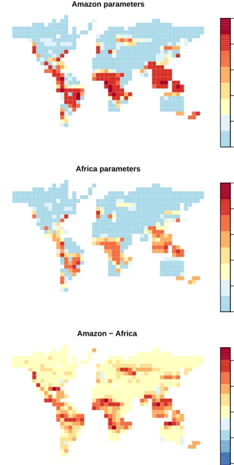
To further explore this difference, we project the “best” set of input parameters, found using the Amazon and African forest to match the simulator against, over a map of the entire FAMOUS land surface. In each case, an independent emula-tor is trained on the ensemble for each grid box. The maps of the mean forest fraction for each parameter set, and the difference between them, are shown in Fig. 12.
Even using the “best” Amazon parameters, the simula-tor underestimates the Amazon coverage in the north-east of South America. This makes it very difficult to simulate a sensible forest fraction, even when overestimating the for-est fraction in places where the simulator does have forfor-est cover.
3.7 History matching allowing for discrepancy in the Amazon
Amazon at various best forest parameters
Broadleaf forest fraction
Em
u
la
te
d
m
e
m
b
e
rs Global
N America SE Asia
Africa
0.0 0.2 0.4 0.6 0.8 1.0
0 1000 2000 3000 4000 5000 6000
Amazon
Other forests at best Amazon parameters
Broadleaf forest fraction
Em
u
la
te
d
m
e
m
b
e
rs
0.0 0.2 0.4 0.6 0.8 1.0
0 2000 4000 6000 8000
Africa
N America
SE Asia
Global
Figure 11.Top panel: forest fraction in the FAMOUS Amazon at the set of parameters where FAMOUS best matches each of the other forest observations. Bottom panel: other forests in FAMOUS at the set where the FAMOUS Amazon best matches observations. Observed forest fractions are shown as marks underneath the his-tograms.
We perform a history match using all of the forest ob-servations, along with a simulator discrepancy term for the Amazon forest. We use the best estimate of the difference between Amazon observations and that simulated by FA-MOUS at the default set of parameters as the best esti-mate of the discrepancy mean. The difference in forest frac-tion at the default parameters is approximately 0.3. Fig-ure 13 shows the histograms of emulated simulator output using this discrepancy term, along with credible estimates for observational uncertainty (1 SD=0.05) and tolerable dis-crepancy uncertainty (1 SD=0.03). The corresponding two-dimensional density plots of NROY emulated input samples can be seen in Fig. 14. The remaining NROY input space represents around 57 % of the original input space defined by the input design, meaning that we have ruled out 43 % of the space. This contrasts with ruling out around 88 % of the space in the initial history match in Sect. 3.1. Marginal histograms of the relative density of NROY points for each individual input parameter (not shown) indicate that no part of the marginal input space is completely ruled out, and so we cannot “constrain” any of the parameters in an individual dimension.
Amazon parameters
0.0 0.2 0.4 0.6 0.8 1.0
Africa parameters
0.0 0.2 0.4 0.6 0.8 1.0
Amazon − Africa
−0.4 −0.2 0.0 0.2 0.4
Figure 12.Maps of mean broadleaf forest fraction, over the “best” set of parameters found for the Amazon (top panel) and the Cen-tral African forest (centre panel). The difference between the two is mapped at the bottom panel.
4 Discussion