conditions in numerical modeling
Menno Fraters1, Cedric Thieulot1, Arie van den Berg1, and Wim Spakman1,2
1Department of Earth Sciences, Faculty of Geosciences, Utrecht University, Utrecht, the Netherlands 2Centre of Earth Evolution and Dynamics (CEED), University of Oslo, Oslo, Norway
Correspondence:Menno Fraters ([email protected]) Received: 29 January 2019 – Discussion started: 14 February 2019
Revised: 10 July 2019 – Accepted: 19 July 2019 – Published: 29 October 2019
Abstract.The Geodynamic World Builder is an open-source code library intended to set up initial conditions for com-putational geodynamic models in both Cartesian and spheri-cal geometries. The inputs for the JavaScript Object Notation (JSON)-style parameter file are not mathematical but rather a structured nested list describing tectonic features, e.g., a con-tinental, an oceanic or a subducting plate. Each of these tec-tonic features can be assigned a specific temperature profile (e.g., plate model) or composition label (e.g., uniform). For each point in space, the Geodynamic World Builder can re-turn the composition and/or temperature. It is written in C++ but can be used in almost any language through its C and Fortran wrappers. Various examples of 2-D and 3-D subduc-tion settings are presented. The Geodynamic World Builder comes with an extensive online user manual.
1 Introduction
Geodynamic modeling has been used in the past four decades to help us better understand the physical processes of Earth’s interior, including large-scale mantle convection and plate tectonics, or detailed processes of crustal deformation. Nu-merical modeling of geodynamic processes involves solving the pertinent partial differential equations (PDEs) of mass, momentum and energy conservation supplemented with rhe-ological laws, material parameters and with an equation of thermodynamic state relating, e.g., density, temperature and pressure (e.g., Gerya, 2010; Schubert et al., 2001). In addi-tion, these PDEs must be constrained by boundary conditions (e.g., velocity, pressure, temperature or heat-flux boundary conditions), which can be time dependent, and by initial
2 Geodynamic World Builder philosophy 2.1 User philosophy
In this section, we describe the philosophy of how tectonic features such as plates, ridges, faults and slabs can be param-eterized by lines and areas that implicitly define volumes to which temperature and composition models can be assigned. A composition is a part of the model that is assigned a par-ticular identifying label and in addition an indicator which is given a value between 0 and 1. This indicator can be used by codes using the GWB output to ascribe physical properties to different model regions.
To minimize user effort, the GWB utilizes a parametriza-tion of 3-D structures by 2-D coordinate input, by defining their (projected) location on the surface. The GWB can be used to create initial models in Cartesian and spherical ge-ometries.
User input files should be specified in JavaScript Ob-ject Notation (JSON) (http://json.org/, last access: 17 Au-gust 2019), which is an internationally standardized language (ISO/IEC 21778). We use a relaxed form of JSON which al-lows comments, NaNs and tailing commas to improve us-ability through RapidJSON (http://rapidjson.org/, last access: 17 August 2019). The user inputs coordinates and can assign particular properties to features such as “linear” for a temper-ature profile or “uniform” for the compositional makeup of the plate. Note that only a subset of the options is mentioned in this paper. We refer to the online Geodynamic World Builder manual (https://geodynamicworldbuilder.github.io, last access: 17 August 2019) for the complete listing.
The GWB uses a hierarchical overlay of features. This means that features defined first are spatially overlain by fea-tures defined later in places where both overlap. The GWB recognizes two types of features: area features and line fea-tures, which will be explained in the following sections. A possible third type of features, point features, will be dis-cussed in Sect. 4.
2.1.1 Continental lithosphere plate
A continental plate is an “area feature” in the GWB and is de-fined by its surface perimeter and its thickness. The perimeter is specified as a list of points which enclose the continental area. Within the defined volume of the continental plate, the GWB offers various options for defining temperature values and compositions. For example, a continental plate can be as-signed multiple layers of different compositions and a linear geotherm that matches a predefined adiabatic mantle temper-ature at the base of the lithosphere. We note that continental lithosphere with a variable thickness is a development for fu-ture releases of the GWB but can be mimicked in the present version by specifying contiguous continental areas with dif-ferent thickness. Also, continental topography is currently not explicitly implemented, but it can be achieved through
a sticky air approach, where air is a composition of varying thickness atop the model (Schmeling et al., 2008; Crameri et al., 2012).
2.1.2 Oceanic lithosphere plate
Like the continental plate, the oceanic plate is parameter-ized as an area feature with a flat surface. We have imple-mented the “plate model” (e.g., Fowler, 2005) for assign-ing an age-dependent temperature to oceanic lithosphere. In Sect. 3.1.2, we will show an example of a ridge–transform system with ridge jumps. The workaround for implementing oceanic bathymetry is the same as that for the continental lithosphere plate.
2.1.3 The mantle
The upper and lower mantles can also be parameterized as an area feature that starts below the lithosphere or at the surface and is overlain by lithosphere in a later building stage. This allows for defining a upper and lower mantle and to insert specific volumetric structures such as large low shear wave velocity provinces (LLSVPs) at the core-mantle boundary in the same way as, for example, an oceanic plate but at depth. In the present version, these mantle features can be assigned a radially uniform, linear or adiabatic temperature profile. Fu-ture versions may include laterally varying temperaFu-ture or compositions, e.g., scaled from seismic tomography models (e.g., Steinberger et al., 2015).
2.1.4 A subducting plate
all examples involving slabs, we will present the equations and implementation here shortly. The temperature in every point in the slab is given by
T (xs, zs)=exp
αg Cpd
θ1+2(θ1−273.15) ∞
X
n=1 (−1)n
nπ
exp
R−R2+n2π2
1 2
xs
sin(nπ zs)
, (1)
where xs is the dimensionless down dip distance xs=xl, wherex is the down dip distance, andl is the thickness of the subducting plate; zs is the dimensionless distance from the bottom of the slab to the top:zs=zl, wherezis distance form the bottom of the slab,αis the thermal expansion coef-ficient,gis the norm of the gravity,Cpis the specific heat at constant pressure,d is the depth below the surface,θ1is the potential mantle temperature at the earths surface, andR is the thermal Reynolds number defined as
R=ρCpvl
2κ , (2)
whereρ is the density,v is the velocity down dip,l is the thickness of the slab, andκ is the thermal conductivity. This formulation is slightly different from the one presented in McKenzie (1970), with the difference that this formulation is not dependent on a constant angle for the slab but directly on the depth, which is what the angle is used for in the original paper.
2.1.5 A fault
To allow for complicated fault shapes (e.g., listric faults), faults are also parameterized as line features. An important difference between faults and subducting plates is that for subducting plates the trench defines the top of the plate at the plate boundary, while for faults the line feature defines the center of the fault with respect to which a fault thickness can be defined.
2.2 Code philosophy
The following design principles define the Geodynamic World Builder:
1. A single text-based input file centered around plate tec-tonic terminology(as explained in Sect. 2.1). The par-ticular syntax is specified in the online manual and will be illustrated with examples below.
systems.
3. Up-to-date user manual and code documentation. Man-ual and doxygen (http://doxygen.nl/, last access: 17 Au-gust 2019) code documentation are provided through https://geodynamicworldbuilder.github.io (last access: 17 August 2019).
4. Safe use in parallel codes: The GWB is split into two phases. The setup phase, encapsulated in the function create_world, is not thread-safe, but upon completion the generated “world object” is thread-safe and can be used to query temperature and compositions in parallel. 5. Readable and extensible code: Following ASPECT (Kronbichler et al., 2012; Heister et al., 2017), we use a plugin system for different parts of the code. Such plug-ins enable users to add functionalities such as plate tec-tonic features or coordinate systems without knowledge of the rest of the code.
6. Version numbering(using Semantic Versioning 2.0.0; https://semver.org/, last access: 17 August 2019). The input file should specify the major version number that must match the version number of the used GWB. Be-fore the release of major version 1, backwards incom-patible changes may be made in minor versions, be-cause they will be beta releases. This implies that the input files for major version 0 also must contain the mi-nor version number. All these features help to ensure reproducibility of results.
3 Using the World Builder
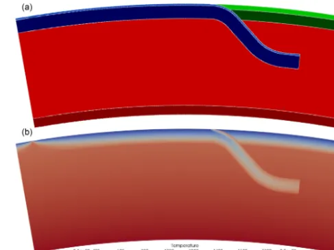
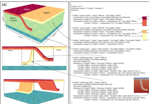
Figure 1.se-2019-24Panel(a)shows the distribution of different compositions through the model domain. The oceanic crust com-position is light blue, the oceanic lithosphere is dark blue, the continental crust is light green, the continental lithosphere is dark green, the upper mantle is light red, and the lower mantle is dark red. Panel(b)shows the temperature distribution (in Kelvin) in the model.
3.1 Stand-alone examples
The GWB has an option to create a ParaView file of the GWB input file. This can be useful for model creation or visual-ization support of presenting geodynamic hypotheses, or for checking the user-designed model prior to using it in a next step, e.g., for creating an initial model for geodynamic mod-eling.
3.1.1 2-D subduction
Here, we show two subduction models, one in Cartesian co-ordinates (Fig. 1) and the same model in spherical (effec-tively cylindrical) coordinates (Fig. 2), which were created through the input files in Appendix A. These input files only differ in the selected coordinate system and whether the sup-plied coordinates are in meters or in degrees. The model has a 95 km thick oceanic plate, of which the top 10 km de-fine the crust, and which turns into a 500 km long subduct-ing slab in the center of the domain. The temperature in the oceanic plate follows the plate model (Fowler, 2005) with a bottom temperature of 1600 K. The slab temperature is com-puted using the McKenzie model for a particular slab history. The model also contains a 100 km thick continental plate of which the top 30 km is crust. Furthermore, the upper and lower mantles are given different compositions and follow a linear temperature profile in the upper mantle from 1600 K
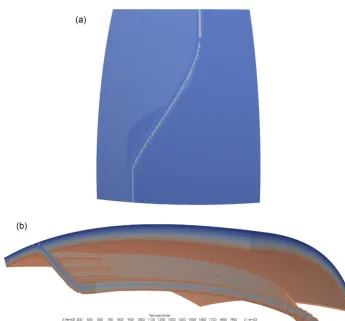
Figure 2.The same as setup as in Fig. 1 but now in spherical geom-etry. Panel(a)shows the composition; panel(b)shows the temper-ature.
at 95 km depth to 1820 K at 660 km depth and in the lower mantle from 1820 at 660 km depth to 2000 at 1160 km depth. This example is created by placing the features in a partic-ular order in the input file. The features overlay, and in this case overwrite, an adiabatic background temperature and all compositions set to zero. This example consists of five fea-tures: an oceanic plate, a continental plate, an upper mantle, a lower mantle and a subducting plate. The first four do not overlap in their input definition, so the order of definition in the Geodynamic World Builder input file does not make a difference in the result. The subducting plate overwrites parts of the oceanic plate, continental plate and the upper mantle, which is effectuated by defining the slab after these three fea-tures. For each feature, temperature and composition models are selected.
3.1.2 3-D ocean spreading
We show in Fig. 3 a 3-D rifting model with two rift systems next to each other. The temperature is defined by the plate model. The mantle is given an adiabatic geotherm defined by θSexp(αgd/Cp), whereθS is the potential surface tempera-ture of the mantle,αis the thermal expansion coefficient,gis the gravitational acceleration,Cpis the specific heat, anddis the depth. The input file of this example consists of the defi-nition of the mantle domain followed by two oceanic plates, which form the two ridge–plate systems. The two oceanic plates are exactly the same, except for the shifted ridge lo-cation. The input file for this example can be found in Ap-pendix B.
3.1.3 3-D subduction
Figure 3.The temperature field of the 3-D two-rift system example. Material with a temperature below 950 K has been omitted in order to better show the rifts. Note the second rift system in the background.
Figure 4. The temperature field of the 3-D subduction example. Note the smooth transition between the upper and lower parts of the subduction system in the top figure and the curved geometry of the slab in panel(b). For visualization purposes, we have omitted the top 25 km of the model in panel(a).
the trench consists of three connected straight lines. To cre-ate a smooth transition between these sections, the user can choose to use a monotone spline interpolation between the coordinates given by the user. This example includes a lin-ear temperature upper and lower mantle as described in the 2-D subduction example. The 95 km thick oceanic plate and the 120 km thick continental plate features are both defined before the subducting plate feature, of which the trench is de-fined along the interface between the two. The slab itself is
95 km thick and consists of four segments: one 200 km long segment which goes from a dip angle of 0 to 45◦ and one 400 km long segment which has an angle of 45◦, one 200 km long segment which goes from 45 to 0◦and one 100 km long
segment with a constant dip angle of 0◦. The input file for
3.2 Using the GWB with SEPRAN
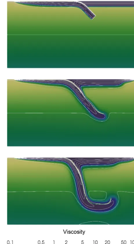
SEPRAN is a general purpose finite element toolkit applied in engineering problems as well as in development of 2-D and 3-D numerical models in geodynamics and planetary science (Chertova et al., 2012, 2014; ˇCížková et al., 2012; van den Berg et al., 2015, 2019; Zhao et al., 2019). The model contains a lithospheric slab subducting under an over-riding plate as shown in Fig. 5. Subduction is driven in a self-consistent way by the ridge push resulting from the thicken-ing of the oceanic plate and the negative buoyancy of the sub-ducted slab. Free-slip impermeable boundary conditions are imposed on the flow. The top of the subducting lithosphere consists of a weak crustal layer, 10 km thick and with a uni-form viscosity of 1020Pa·s. This weak crustal layer plays an essential role in preventing the locking of the subducting lithosphere with the overriding plate that would stop the sub-duction process (Androviˇcová et al., 2013). The mantle un-derlying the crust has a temperature- and pressure-dependent viscosity with an Arrhenius-type parametrization representa-tive of diffusion creep in olivine under upper mantle pres-sure and temperature conditions. Viscosity is modeled as a material property for the crustal layer material and the man-tle material. Material transport is implemented using particle tracers that are advected by the convective flow. The medium is described as a mechanical mixture of materials with con-trasting properties.
A 2-D rectangular domain of 1000 km depth and 2000 km width is used. The initial thermal and composition state is created using the Fortran wrapper of the GWB library. The GWB tool is called in a loop over all nodal points of the finite element method (FEM) mesh to define the initial temperature field for the subsequent convection calculations. In a similar way, the material distribution of the initial state is defined by calling the composition function of the GWB library in a program loop over particle tracers. The input file for this example can be found in Appendix D.
3.3 Using the GWB with ELEFANT
ELEFANT is a 2-D/3-D finite element code for geodynamic problems (Maffione et al., 2015; Lavecchia et al., 2017; Thieulot, 2017; Plunder et al., 2018) written in Fortran. It principally relies on bi-/trilinear velocity-constant pressure elements and uses the marker-in-cell technique to track ma-terials. In order to demonstrate the GWB flexibility of use, a 3-D double subduction setup was created with the Fortran wrapper of the GWB (see Fig. 6): a composition between 1 and 6 was then easily assigned to all markers (two differ-ent oceanic crusts and oceanic lithospheres, one upper man-tle and one lower manman-tle) and a temperature based on the McKenzie model (McKenzie, 1970) was prescribed onto the FE mesh, as shown in Fig. 7.
The domain is a Cartesian box with dimensions 2000× 2000×800 km and the finite element mesh counts 120×
Figure 5.Dimensionless viscosity field in log scale superimposed with 10 (dimensionless) temperature (between 0 and 0.82) isocon-tours.
120×50=720 000 elements. Each element contains 64 ran-domly distributed markers. Free-slip boundary conditions are imposed at the bottom (z=0), top (z=Lz) and sides
(y=0 and y=Ly) of the domain. The other two sides,
x=0 and x=Lx, are a mix of free-slip (for z <100 or
z >690 km) and open boundary conditions (for 100< z < 690 km) (Chertova et al., 2012). The input file for this exam-ple can be found in Appendix E.
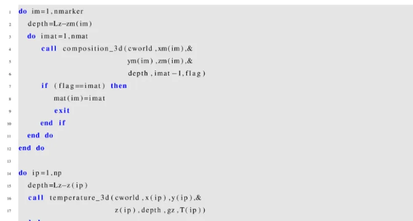
Figure 6.Example ELEFANT query routine using the GWB-supplied Fortran wrappers composition_3d() and temperature_3d():(a)a loop runs over all markers and determines for each the composition at its location;(b)a loop runs over all grid points and the GWB returns its temperature as a function of their spatial coordinates.
Figure 7. (a)Markers for five compositions (the mantle markers have been left out for ease of visualization) with the resulting velocity field.
(b)Temperature field.
3.4 Using the GWB with ASPECT
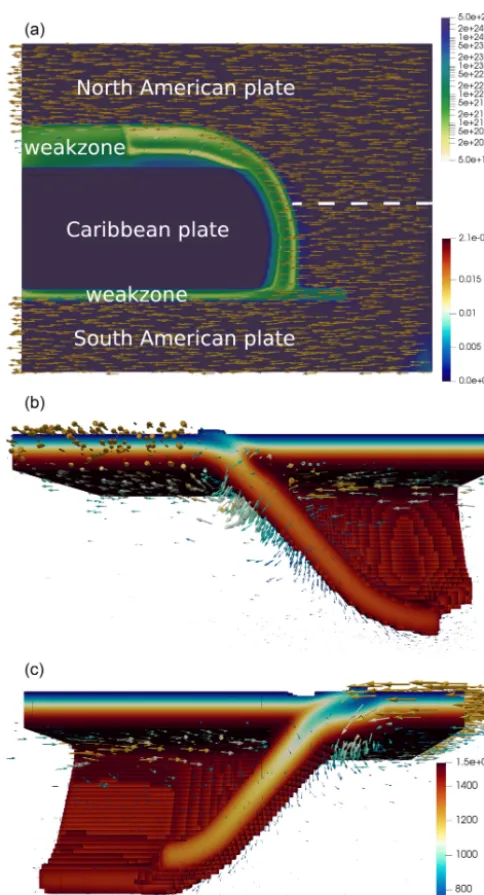
ASPECT is an open-source community FEM designed for geodynamic problems (Heister et al., 2017; Kronbichler et al., 2012). The model which was run with ASPECT is a 3-D Cartesian model of a curved subduction system similar to the plate tectonic setting of the Lesser Antilles subduc-tion of the eastern Caribbean region. The lithosphere con-sists of a strong zero-velocity Caribbean upper plate, sur-rounded by an oceanic North American plate to the north and northeast and the oceanic–continental South American plate to the south and southeast. In the model, the North American and South American plates move west at a aver-age rate over the past 5 Myr of 1.4 cm yr−1 relative to the Caribbean plate (Boschman et al., 2014). The Lesser Antilles trench curves around the east and north of the Caribbean plate. To the south, the Caribbean plate is partially
decou-pled from the South American plate by a 50 km wide weak zone. To the northwest, a 250 km wide weak zone, from the western end of the trench to the western edge of the model, partially decouples the North American plate from the Caribbean plate. Below the lithosphere, the sidewalls are open (Chertova et al., 2012, 2014) allowing for horizontal in-/outflow of mantle material. From 660 km down, a denser and more viscous material has been prescribed to delay sink-ing of the slab into the lower mantle. The top boundary is a free surface (Rose et al., 2017) and the bottom boundary has a prescribed zero velocity. The result of about 2.5 million years of evolution is shown in Fig. 9.
Figure 8.Connection between the GWB input file(a)and the resulting marker fields(b). Small upper inserts in panel(b)show each plate layering, while the bottom insert shows the temperature field zoomed in on slab B.
3.5 Performance
The finite element mesh used in the example of Sect. 3.4 is built in several steps by ASPECT: the code starts with a reg-ular grid and allows adaptive mesh refinement to take place one level at the time. Each step of this process calls the GWB library. The first step generates a grid counting 28 000 el-ements and reports a total setup time for the initial condi-tions of 3.6 s on 480 MPI processes. The second step mesh counts 99 000 elements, while the setup of the initial condi-tions took (cumulatively) 10 s. The third step sees the number of element jump to about 560 000 elements, while its total (cumulative) time to setup the initial conditions remains low at about 36 s. This figure represents about 0.7 % of the total wall time of the first time step and a negligible portion of the total wall time of the 20 Myr long simulation.
4 Discussion
We presented the Geodynamic World Builder version 0.2.0 as a tool for constructing 2-D and 3-D initial models of geo-dynamic settings involving crust/lithosphere, plate
Figure 9.The 3-D ASPECT Caribbean example after 2.5 million years of evolution. The top image is a top view of the model where the top 50 km section is removed and where the viscosity field is shown with the velocity field indicated by the arrows. The bottom two figures are cutouts of the temperature field between 600 and 1535 K, showing in color the temperature (T), and with arrows the velocity fields, highlighting the velocity field in the slab and litho-sphere.
Appendix A: 2-D subduction examples A1 Cartesian input file
A2 Spherical input file
Appendix B: 3-D ocean spreading example input file
Appendix F: ASPECT 3-D curved subduction
Author contributions. MF wrote the code, the documentation and most of the paper, and coordinated with the other authors. CT pro-vided advice on algorithms and general coding, coupled the code ELEFANT to the GWB, documented that, wrote the section related to ELEFANT and provided feedback on the rest of the paper. AvdB coupled SEPRAN to the GWB, documented that and wrote the sec-tion related to SEPRAN. WS provided advice during the project and contributed to the overall setup and writing of the paper.
Competing interests. The authors declare that they have no conflict of interest.
Acknowledgements. Menno Fraters acknowledges constructive feedback from the ASPECT community and especially from Timo Heister, Wolfgang Bangerth and Rene Gassmöller. The au-thors also acknowledge constructive proofreading by Robert My-hill, Henry Brett and Lucas van de Wiel. Menno Fraters and Cedric Thieulot are indebted to the Computational Infrastructure for Geo-dynamics (CIG) for their recurring participation in the ASPECT hackathons, during which the foundation of this work was laid out. This work is funded by the Netherlands Organisation for Scientific Research (NWO), as part of the Caribbean Research program (grant no. 858.14.070) and partly supported by the Research Council of Norway through its Centres of Excellence funding scheme, project no. 223272. Data visualization is carried out with ParaView soft-ware https://paraview.org/ (last access: 17 August 2019).
Financial support. This research has been supported by the Nether-lands Organisation for Scientific Research (NWO) (grant no. 858.14.070) and the Research Council of Norway (grant no. 223272).
Review statement. This paper was edited by Taras Gerya and re-viewed by Fabio A. Capitanio and one anonymous referee.
References
Alisic, L., Gurnis, M., Stadler, G., Burstedde, C., and Ghat-tas, O.: Multi-scale dynamics and rheology of man-tle flow with plates, J. Geophys. Res., 117, B10402, https://doi.org/10.1029/2012JB009234, 2012.
Androviˇcová, A., ˇCížková, H., and van den Berg, A.: The ef-fects of rheological decoupling on slab deformation in the Earth’s upper mantle, Stud. Geophys. Geod., 57, 460–481, https://doi.org/10.1007/s11200-012-0259-7, 2013.
Billen, M. and Arredondo, K.: Decoupling of plate-asthenosphere motion caused by non-linear viscosity during slab folding in the transition zone, Phys. Earth. Planet. Inter., 281, 17–30, 2018. Boschman, L. M., van Hinsbergen, D. J., Torsvik, T. H., Spakman,
W., and Pindell, J. L.: Kinematic reconstruction of the Caribbean region since the Early Jurassic, Earth-Sci. Rev., 138, 102–136, https://doi.org/10.1016/j.earscirev.2014.08.007, 2014.
Brune, S. and Autin, J.: The rift to break-up evolution of the Gulf of Aden: Insights from 3D numerical lithospheric-scale modelling, Tectonophysics, 607, 65–79, 2013.
Chertova, M. V., Geenen, T., van den Berg, A., and Spak-man, W.: Using open sidewalls for modelling self-consistent lithosphere subduction dynamics, Solid Earth, 3, 313–326, https://doi.org/10.5194/se-3-313-2012, 2012.
Chertova, M., Spakman, W., Geenen, T., van den Berg, A., and van Hinsbergen, D.: Underpinning tectonic reconstructions of the western Mediterranean region with dynamic slab evolution from 3-D numerical modeling, J. Geophys. Res., 119, 5876– 5902, https://doi.org/10.1002/2014JB011150, 2014.
ˇ
Cížková, H., van den Berg, A., Spakman, W., and Matyska, C.: The viscosity of the earth’s lower mantle inferred from sinking speed of subducted lithosphere, Phys. Earth. Planet. Inter., 200–201, 56–62, 2012.
Crameri, F., Schmeling, H., Golabek, G., Duretz, T., Orendt, R., Buiter, S., May, D., Kaus, B., Gerya, T., and Tackley, P.: A com-parison of numerical surface topography calculations in geody-namic modelling: an evaluation of the ’sticky air’ method, Geo-phy. J. Int., 189, 38–54, 2012.
Duretz, T., Gerya, T., and Spakman, W.: Slab detachment in lat-erally varying subduction zones: 3-D numerical modeling, Geo-phys. Res. Lett., 41, 1951–1956, 2014.
Fowler, C.: The Solid Earth: An Introduction to Global Geophysics, Cambridge University Press, UK, 2005.
Fraters, M.: The Geodynamic World Builder (Version v0.2.0), Zen-odo, https://doi.org/10.5281/zenodo.3517132, last access: 23 Oc-tober 2019.
Gerya, T.: Dynamical instability produces transform faults at mid-ocean ridges, Science, 329, 1047–1050, 2010.
Heister, T., Dannberg, J., Gassmöller, R., and Bangerth, W.: High Accuracy Mantle Convection Simulation through Modern Nu-merical Methods, II: Realistic Models and Problems, Geo-phy. J. Int., 210, 833–851, 2017.
Holt, A., Becker, T., and Buffett, B.: Trench migration and overrid-ing plate stress in dynamic subduction models, Geophy. J. Int., 201, 172–192, 2015.
Jadamec, M. and Billen, M.: Reconciling surface plate motions with rapid three-dimensional mantle flow around a slab edge, Nature, 465, 338–341, 2010.
Jadamec, M. and Billen, M.: The role of rheology and slab shape on rapid mantle flow: Three-dimensional numerical mod-els of the Alaska slab edge, J. Geophys. Res., 117, B02304, https://doi.org/10.1029/2011JB008562, 2012.
Kiraly, A., Capitanio, F., Funiciello, F., and Faccenna, C.: Subduc-tion zone interacSubduc-tion: Controls on arcuate belts, Geology, 44, 715–718, https://doi.org/10.1130/G37912.1, 2016.
Kronbichler, M., Heister, T., and Bangerth, W.: High accuracy man-tle convection simulation through modern numerical methods, Geophy. J. Int., 191, 12–29, 2012.
Lavecchia, A., Thieulot, C., Beekman, F., Cloetingh, S., and Clark, S.: Lithosphere erosion and continental breakup: Interaction of extension, plume upwelling and melting, Earth Planet. Sc. Lett., 467, 89–98, 2017.
Leng, W. and Gurnis, M.: Subduction initiation at relic arcs, Geo-phys. Res. Lett., 42, 7014–7021, 2015.
effect of obliquity on temperature in subduction zones: in-sights from 3-D numerical modeling, Solid Earth, 9, 759–776, https://doi.org/10.5194/se-9-759-2018, 2018.
Rose, I., Buffet, B., and Heister, T.: Stability and accuracy of free surface time integration in viscous flows, Phys. Earth. Planet. In-ter., 262, 90–100, 2017.
Schellart, W. and Moresi, L.: A new driving mechanism for backarc extension and backarc shortening through slab sinking induced toroidal and poloidal mantle flow: Results from dynamic sub-duction models with an overriding plate, J. Geophys. Res., 118, 1–28, 2013.
Schellart, W. P.: Andean mountain building and magmatic arc migration driven by subduction-induced whole mantle flow, Nat. Commun., 8, https://doi.org/10.1038/s41467-017-01847-z, 2017.
Schmeling, H., Babeyko, A., Enns, A., Faccenna, C., Funiciello, F., Gerya, T., Golabek, G., Grigull, S., Kaus, B., Morra, G., Schmalholz, S., and van Hunen, J.: A benchmark comparison of spontaneous subduction models – Towards a free surface, Phys. Earth. Planet. Inter., 171, 198–223, 2008.
Schubert, G., Turcotte, D., and Olson, P.: Mantle Convection in the Earth and Planets, Cambridge University Press, Cambridge, 2001.
van den Berg, A., Segal, G., and Yuen, D.: SEPRAN: A Versatile Finite-Element Package for a Wide Variety of Problems in Geo-sciences, J. Earth Sci., 26, 89–95, 2015.
van den Berg, A., Yuen, D., Umemoto, K., Jacobs, M., and Wentz-covitch, R.: Mass-dependent dynamics of terrestrial exoplanets using ab initio mineral properties, Icarus, 317, 412–426, 2019. Yamato, P., Husson, L., Braun, J., Loiselet, C., and
Thieu-lot, C.: Influence of surrounding plates on 3D sub-duction dynamics, Geophys. Res. Lett., 36, L07303, https://doi.org/10.29/2008GL036942, 2009.
Zhao, Y., de Vries, J., van den Berg, A., Jacobs, M., and van Westrenen, W.: The participation of ilmenite-bearing cu-mulates in lunar mantle overturn, Earth Planet. Sc. Lett., https://doi.org/10.1016/j.epsl.2019.01.022, 2019.