Automatically delineating the calving front of Jakobshavn Isbræ from multitemporal TerraSAR-X images: a deep learning approach

(1)

Automatically delineating the calving front of Jakobshavn Isbræ

from multitemporal TerraSAR-X images: a deep learning approach

Enze Zhang, Lin Liu, and Lingcao Huang

Earth System Science Programme, Faculty of Science, The Chinese University of Hong Kong, Hong Kong, China Correspondence:Enze Zhang ([email protected])

Received: 18 January 2019 – Discussion started: 7 February 2019

Revised: 23 May 2019 – Accepted: 6 June 2019 – Published: 28 June 2019

Abstract. The calving fronts of many tidewater glaciers in Greenland have been undergoing strong seasonal and in-terannual fluctuations. Conventionally, calving front posi-tions have been manually delineated from remote sensing images. But manual practices can be labor-intensive and time-consuming, particularly when processing a large num-ber of images taken over decades and covering large areas with many glaciers, such as Greenland. Applying U-Net, a deep learning architecture, to multitemporal synthetic aper-ture radar images taken by the TerraSAR-X satellite, we here automatically delineate the calving front positions of Jakobshavn Isbræ from 2009 to 2015. Our results are con-sistent with the manually delineated products generated by the Greenland Ice Sheet Climate Change Initiative project. We show that the calving fronts of Jakobshavn’s two main branches retreated at mean rates of −117±1 and−157± 1 m yr−1, respectively, during the years 2009 to 2015. The interannual calving front variations can be roughly divided into three phases for both branches. The retreat rates of the two branches tripled and doubled, respectively, from phase 1 (April 2009–January 2011) to phase 2 (January 2011– January 2013) and then stabilized to nearly zero in phase 3 (January 2013–December 2015). We suggest that the re-treat of the calving front into an overdeepened basin whose bed is retrograde may have accelerated the retreat after 2011, while the inland–uphill bed slope behind the bottom of the overdeepened basin has prevented the glacier from retreat-ing further after 2012. Demonstratretreat-ing through this successful case study on Jakobshavn Isbræ and due to the transferable nature of deep learning, our methodology can be applied to many other tidewater glaciers both in Greenland and else-where in the world, using multitemporal and multisensor re-mote sensing imagery.

1 Introduction

Glacier retreating is one of the processes that control the re-cent speedups of Greenland’s tidewater glaciers (King et al., 2018). As a glacier retreats, it accelerates to compensate for the loss of downstream buttress. Glacier dynamic instabil-ities, as suggested decades ago by Meier and Post (1987), play an essential role as the glaciers retreat over depres-sions in the bedrock topography. For example, Joughin et al. (2008a) indicated that dynamic instabilities caused Hel-heim and Kangerdlugssuaq glaciers to speed up as they re-treated into an overdeepened basin whose bed is retrograde between 2001 and 2006. Examining 276 marine-terminating outlet glaciers, Bunce et al. (2018) concluded that bed geom-etry is an important control on the timing and magnitude of glacier retreat.

An accurate and detailed quantification of calving front variations would improve our understanding of the con-trolling mechanisms of glacier retreat. Moreover, observa-tions of retreat may serve as initial indicators for other dy-namic variations such as the glacier acceleration (Moon and Joughin, 2008). Calving front positions are influenced by a range of forces including ice mélange buttressing, increased runoff, and ocean-driven melt (Moon et al., 2015; Fried et al., 2018). Nevertheless, the mechanisms behind the numer-ous and complex controls on front positions are not yet fully understood.

(2)

1730 E. Zhang et al.: Automatically delineating the calving front of Jakobshavn Isbræ

al. (1996) designed a method to extract the ice sheet margin by applying the Roberts edge extractor to ERS-1 synthetic aperture radar (SAR) images. Seale et al. (2011) automati-cally identified glacier calving fronts from daily MODIS im-ages by combining Sobel and brightness profiling methods. With low computational complexity requiring no training and little memory resources, these feature-extracting meth-ods are promising but require extensive prior knowledge and experience. The deep learning method has also been ap-plied to delineate the calving front positions. Mohajerani et al. (2019) have applied the U-Net architecture to Landsat-5, 7, and 8 images over Jakobshavn, Sverdrup, Kangerlussuaq, and Helheim glaciers.

Deep learning can solve more complex problems with lit-tle prior knowledge required and take advantage of increased data volume (LeCun et al., 2015). With the continuous ac-cumulation in the past decades and in recent space missions, the data volume of remote sensing imagery in the polar re-gions has increased dramatically. Moreover, glacier systems are complex, as conditions such as weather and glacier dy-namic behaviors vary from place to place and from season to season. There are therefore obvious advantages to applying deep learning techniques to automatically extract glaciologi-cal features from the available big data.

Here we aim to design a method to automatically delin-eate a glacier calving front from multitemporal TerraSAR-X (TSTerraSAR-X) images based on deep convolution neural networks (DCNNs). More specifically, we delineate the glacier calving front of Jakobshavn Isbræ (Fig. 1a) and quantify its seasonal and interannual variations. With this new set of observations, we investigate the possible link between calving front varia-tions and bed elevation.

DCNNs are a class of the deep learning methods and have made important breakthroughs in image processing. DCNNs can discover both low-level (e.g., edges, corners, and lines) and midlevel features (e.g., shapes, sizes, and locations) (Sun et al., 2014; Zhang et al., 2015). Recently, some studies have used DCNNs on high-resolution SAR images to perform classification tasks (Geng et al., 2015; Huang et al., 2017). These studies unanimously agree that DCNNs outperform traditional classification methods on SAR images.

We use TSX images due to their high temporal resolu-tion (11 d), high spatial resoluresolu-tion (3.3 to 3.5 m), and ability to penetrate cloud cover. These high-temporal-resolution im-ages have been acquired in all seasons and allow us to investi-gate calving front variations with a high degree of continuity and consistency. With these high-spatial-resolution images, we can easily digitize the calving fronts (known as ground truth in the context of deep learning) and verify the accuracy of the DCNN. Using SAR images can avoid the cloud cover problem associated with optical images such as the Landsat-8 image shown in Fig. 1b.

2 Jakobshavn Isbræ

Jakobshavn Isbræ, located in central-west Greenland, is one of the largest and fastest tidewater glaciers in the world. In Jakobshavn, the ice flows westward to the ocean and divides into two branches near the coast (Fig. 1a). Before summer 2004, these two branches merged and flowed into the Kangia Fjord. Afterwards, as the glacier retreated, the two branches became disconnected (Bondzio, 2017). During the past few years, Jakobshavn Isbræ has undergone dramatic accelera-tion as the glacier has retreated and thinned (Joughin et al., 2008c, 2012). Jakobshavn’s calving front retreated 16 km be-tween 2002 and 2008 (Rosenau et al., 2013). This glacier alone has contributed nearly 1 mm to the global sea level rise from 2000 to 2011 (Howat et al., 2011).

Observations have shown that the calving front variations were correlated with the glacier velocity changes in Jakob-shavn Isbræ. In 1998, the glacier sped up by 18 % in its frontal regions, coinciding with the initial retreat of the ice tongue (Thomas, 2004; Luckman and Murray, 2005). The glacier doubled its speed by spring 2003, when nearly the entire floating ice tongue had disintegrated (Joughin et al., 2004). After the loss of this ice tongue, the glacier’s veloc-ity fluctuated seasonally from 2004 to 2007 (Joughin et al., 2008b). The glacier slowed down when it was advancing and sped up when it was retreating (Joughin et al., 2012).

The variations of Jakobshavn’s calving front are also strongly influenced by the presence of ice mélange, namely a mixture of calved icebergs and sea ice (Fig. 1a). The sea-sonal variation of the calving front in Jakobshavn Isbræ is well correlated with the growth and recession of sea ice in the Kangia Fjord (Sohn et al., 1998; Joughin et al., 2008c). Temporal variations of the ice mélange strength can also con-trol the timing of calving events and influence the evolution of the calving front position (Amundson et al., 2010).

(3)

Figure 1. (a)TerraSAR-X image taken on 11 July 2015 showing the frontal area of Jakobshavn Isbræ. Its two branches are labeled as “A” and “B”. The green lines indicate the location of the bed elevation profiles shown in Fig. 8.(b)Landsat-8 image taken on 13 July 2015. The white box shows the area illustrated in(a).

3 TerraSAR-X images and preprocessing

The German SAR satellite TerraSAR-X was launched in June 2007 and carries an X-band SAR sensor. In this study, we use TSX images taken in both ascending and descending orbits and in stripmap imaging mode. We use the enhanced-ellipsoid-corrected (EEC) products, which are multilooked, projected, and resampled to the WGS84 reference ellipsoid. We use 159 images in total, taken between 16 April 2009 and 23 December 2015 (listed in Table S1 in the Supplement). We apply three preprocessing procedures including despeck-ling, multilooking, and regeoreferencing. Figure 2 shows an illustrative example of our preprocessing workflow, which we will describe below in detail.

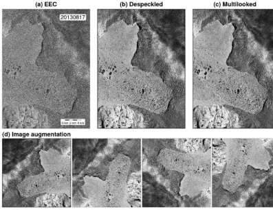
Because the quality of SAR images is adversely affected by the speckle noise (Fig. 2a), we apply the median blur filter to mitigate the speckle noise (Fig. 2b) and then multilook the filtered images to reduce their size by 25 times (Fig. 2c). The median blur filter is widely used in image processing and is particularly effective for speckle noise. With the despeckled images, we average five neighboring pixels (vertically and horizontally) by using the Geospatial Data Abstraction Li-brary (GDAL) package (https://gdal.org/, last access: 17 Jan-uary 2019). Moreover, both despeckling and multilooking can smooth images without the loss of essential information for delineating the calving fronts. After despeckling and mul-tilooking, the pixel size of our images is 6 m.

We choose the EEC products because they include to-pographic correction and are the standard geocoded

prod-ucts of TSX (Roth et al., 2004). However, even for the EEC products, we observe that the geocoding information for our study area is inaccurate. First, overlaying the EEC images on Google Earth, we note obvious offsets between these two. Second, the geocoding information is inconsistent in different orbit directions of EEC products. Therefore, we need to regeoreference the EEC products. For the images we have, we observe that the images in the same orbit direction have identical geometry. Based on this observation, we as-sume that the differences between the EEC products and the Google Earth images are systematic, namely that they are consistent for the EEC products in the same orbit direction. We correct the geocoding information of the EEC products using 16 ground control points on Google Earth images, in-cluding the center of lakes and cross sections of the bedrock, due to their stability and ease of identification. For all the EEC products in the same orbit direction, we apply the same thin plate spline transformation using the GDAL package.

4 Deep learning and postprocessing

(4)

Figure 2. A set of examples of TerraSAR-X data preprocessing and preparation, including the(a)enhanced-ellipsoid-corrected (EEC) product,(b)despeckled image after reducing the speckle noise,(c)multilooked image after decreasing the image size, and(d)images after vertically flipping and rotating(c)by 90, 180, and 270◦, respectively. For ease of presentation, the images in(d)are not to scale with(a)–(c).

the best methods in image segmentation (Ronneberger et al., 2015). This network is fast, taking less than a second on a mainstream graphics processing unit (GPU) to segment a 512 pixels×512 pixels image. The U-Net architecture con-sists of a contracting path and an expansive path (Fig. S1 in the Supplement). The contracting path consists of repeated application of two 5×5 convolution layers, each followed by a batch normalization layer and a leaky rectified linear unit (LeakyReLU) activation function, as well as 2×2 max pool-ing operation for downsamplpool-ing feature maps and doublpool-ing the number of feature channels. Every step in the expansive path consists of a 4×4 up-convolution layer that upsamples the feature map and halves the number of feature channels, a concatenation with the corresponding feature map from the contracting path and two 5×5 convolution layers, each followed by a batch normalization layer and a LeakyReLU activation function. The final layer is a 3×3 convolutional layer with the sigmoid activation function to get the final seg-mentation patch. We utilize relatively large convolution ker-nel size (5 by 5) to obtain smoother calving fronts. We use LeakyReLU activation functions with a slope of 0.1 below zero, which allows for a small, nonzero gradient when the unit is not active (Maas et al., 2013), making optimization

potentially more robust. We use binary cross entropy (BCE) between the ground truth images and the network outputs to measure the training error because it avoids the problem of slow learning (the training loss decreases slowly) (Goodfel-low et al., 2016). We use adaptive moment estimation max (AdaMax) (Kingma and Ba, 2015) as the optimizer with a learning rate of 0.0001 and an L2 regularization factor of 0.00001.

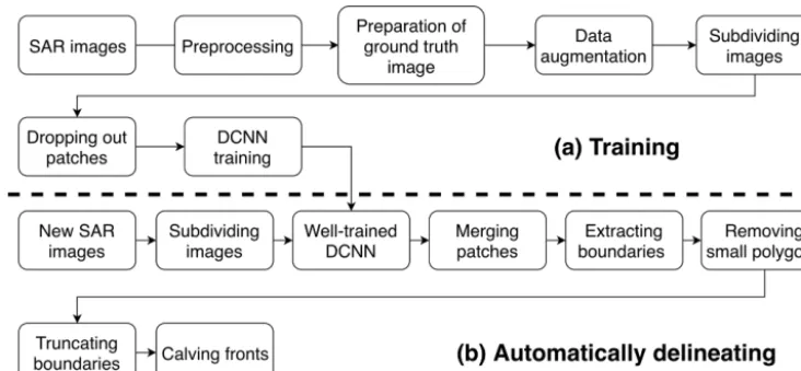
The proposed framework for using deep learning to de-lineate the calving fronts is summarized in Fig. 3. We sep-arate all the SAR images into a training–validation dataset (75 images) and a test dataset (84 images) (Table S1). In the training–validation dataset, we randomly choose 90 % as training data and take the rest as validation data. The valida-tion dataset is for minimizing overfitting and tuning the hy-perparameters of the network such as learning rate and kernel size.

(5)

Figure 3.Diagram of the proposed framework. Details are described in Sects. 3 and 4.

images are derived by converting the vector of manually de-lineated calving fronts to rasters using GDAL. Manual delin-eation is simple on most TSX images. However, it is chal-lenging to delineate the calving fronts on the few TSX im-ages acquired in winter and spring because the boundaries are obscured due to snow cover and sea ice bonding. For each of these obscure images, we use its temporally closest image with a clear calving front as a reference and require that our manually delineated fronts are smooth (Fig. S3).

To ensure the effectiveness and accuracy of deep learn-ing for a set of SAR images taken in all seasons spannlearn-ing 7 years, it is important to prepare a sufficiently diverse train-ing dataset. We include at least one image in each month into the training dataset to represent various conditions related to radar backscatter and image texture. First, radar backscatter can vary with the dielectric properties of the surface scatter-ers in the study area due to changes in snow cover, wetness, and variations in geometric properties such as roughness, grain size, and internal structure (Fahnestock et al., 1993). Since our study area is in the ablation region, backscatter in-creases in winter because of dry snow cover and dein-creases in summer due to snow melting. Second, the seasonal and in-terannual variations of the ice mélange condition can change the image texture. Sea ice formation in winter solidifies ice mélange, while ice mélange weakens in summer, resulting in freely floating icebergs (Amundson et al., 2010; Xie et al., 2016).

We also perform data augmentation to enrich our training dataset. We adopt the following two strategies. First, we ver-tically flip and rotate our training images by 90, 180, and 270◦, respectively, to constitute many possible locations of the calving front in the study area (Fig. 2d). Second, we ap-ply a 2 % linear stretch to the training images to enhance the edges. For all the values between the 2nd and 98th percentiles of the pixel value histogram, we linearly stretch them to the range between 0 and 255. The values lower than the 2nd

per-centile are set to zero, and the values larger than the 98th percentile are set to 255.

We subdivide each image (3565 pixels×1634 pixels) in the training dataset into small patches (960 pixels×720 pixels). Otherwise, the resolution would be limited by the GPU mem-ory. We split images with overlaps and obtain 36 414 patches in total. Such a strategy allows a seamless segmentation after merging, which reduces the edge effect. A larger patch size can also better mitigate the edge effect. A common train-ing strategy in deep learntrain-ing is to train several traintrain-ing ex-amples as a batch each time instead of training the whole dataset. With a given GPU memory, a smaller patch size al-lows more items in a batch, which increases the efficiency and improves the accuracy of the gradient estimation at each step. To strike a balance between edge effect and batch size, we choose 960 pixels×720 pixels as our patch size, and the batch size is three.

Due to different computational time used in training and automatic delineation, the overlap areas between adjacent patches are set differently in the training and the test datasets. Taking the GPU we use as an example, training the network takes more time (80 h) than automatic delineation (20 min) after the network is well trained. Therefore, we split the train-ing images with smaller overlap (two-thirds of the patch size) to save computational power and split the test images with larger overlap (four-fifths of the patch size) to make denser samplings so that the results become more robust.

(6)

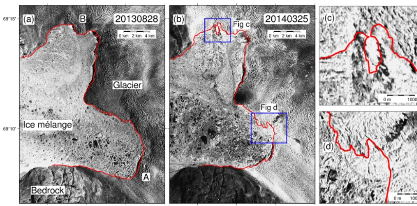
Figure 4.Examples of(a)superior and(b)inferior delineation from our deep-learning-based method. In both(a)and(b), the red line shows the calving front delineated by the network.(c)and(d)show the zoomed-in figure of the obscure calving front positions within the blue boxes in(b).

Training the network starts with initializing all weights as zero. We stop the training when the validation error starts to increase for five consecutive epochs. After the training, we first subdivide each test TSX image into small patches and use the well-trained network to segment all the patches into ice mélange and nonice mélange classes. Then, we merge the segmented patches (binary images with a pixel value of one or zero) into a single segmentation image by averaging the overlaps. After merging, if the pixel value is larger than 0.5, we consider the pixel to be in a nonice mélange region. We use GDAL to convert the segmentation image into a vector, which contains a large polygon constituted by both the calv-ing front and the image border, as well as small isolated poly-gons caused by erroneous segmentation. After removing the small polygons and truncating the large polygon to separate the calving front from the image border, we finally obtain the calving front for each image.

Using the postprocessed delineation results, we can quan-tify the temporal calving front variations of both branches. Taking the earliest calving front (16 April 2009) as the ref-erence, we calculate the enclosed area bounded by the refer-ence and the calving front in a given TSX image. We adopt these metrics of area changes because they take both calving front position and shape into account.

5 Data validation and error estimation

Our results are validated by calving front products from the Greenland Ice Sheet Climate Change Initiative (CCI) project (http://products.esa-icesheets-cci.org, last access: 8 Octo-ber 2018). The CCI calving fronts are derived by manual

de-lineation using ERS and Sentinel-1 SAR, as well as Landsat-5, 7, and 8 optical imagery. We validate our results in the following two aspects.

First, the validation of the regeoreferencing (Sect. 3) is de-rived by directly comparing the manually delineated calving fronts obtained from this study and the CCI products. The calving fronts from these two datasets should be on the same date, and therefore only six calving fronts are compared. We manually delineate the calving fronts from the TSX image af-ter regeoreferencing and then calculate the averaged width of the enclosed area bounded by both of the calving fronts from these two datasets. The mean difference is 104 m (equiva-lent to∼17.3 pixels) (Table S2 and Fig. S4). Several reasons could cause such a seemingly large difference. The geocod-ing information of the CCI products also has uncertainties. Moreover, manual delineations from both the CCI and ours are subjected to image quality and the different criteria we adopt for front delineation. To measure the manual eation error, we have another investigator to manually delin-eate the abovementioned six calving fronts again. By com-paring the two sets of independent delineation results, we ob-tained a mean difference of 33 m (equivalent to∼5.5 pixels) (Table S2).

Second, the difference of calving front variations between ours and the CCI presents an overall validation that sums up both regeoreferencing and network-delineation uncertainties. We quantify the calving front variations of the CCI products with the same method and reference used in our results. Fi-nally, we calculate the difference between these two varia-tions in terms of both area and equivalent length.

(7)

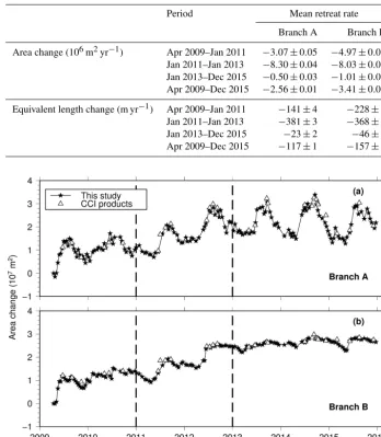
train-Area change (106m2yr−1) Apr 2009–Jan 2011 −3.07±0.05 −4.97±0.09 Jan 2011–Jan 2013 −8.30±0.04 −8.03±0.07 Jan 2013–Dec 2015 −0.50±0.03 −1.01±0.03 Apr 2009–Dec 2015 −2.56±0.01 −3.41±0.01

Equivalent length change (m yr−1) Apr 2009–Jan 2011 −141±4 −228±9 Jan 2011–Jan 2013 −381±3 −368±5 Jan 2013–Dec 2015 −23±2 −46±2 Apr 2009–Dec 2015 −117±1 −157±1

Figure 5.Time series of calving front variations (in area changes) of branches A and B from our deep learning method (stars) and the Greenland Ice Sheet CCI project (triangles). Dashed vertical lines divide the time series into three separate phases (see text).

ing, the test error is for calving front delineation. We mea-sure the test error by calculating the averaged width of the enclosed area bounded by the manually delineated and the network-delineated calving fronts (Fig. S5).

6 Results

We present our results in the following order: (1) the network-delineated calving fronts from 16 April 2009 to 23 December 2015, which are shown in a movie (Movie S1 in the Supplement); (2) two examples of our automatically delineated calving fronts (i.e., results in test dataset) (Fig. 4); (3) retreat rates (Table 1) and time series of calving front

vari-ations (Fig. 5); (4) interannual calving front variation (Figs. 6 and 7).

(8)

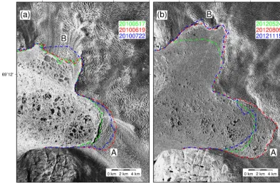
Figure 6.Two examples showing the asynchronous behaviors of branches A and B.(a)Branch A began to retreat in May 2010, while Branch B started to retreat 1 month later.(b)Branch A’s calving front underwent strong variation between August and November 2012, whereas Branch B’s calving front was relatively stable. The magenta line in both(a)and(b)shows the calving front position just before the annual retreat.

Overall, our results agree well with the CCI products (Fig. 5). The area difference is 2.14×106m2, and the equiv-alent length difference is 73 m. Moreover, our results have a higher temporal resolution (about two measurements ev-ery month) than the CCI products (about four measurements every year). Therefore, we can observe the seasonal and interannual variations more clearly. Based on our results, branches A and B retreated from 2009 to 2015 with linear trends of−117±1 and−157±1 m yr−1, respectively. The in-terannual variation can be roughly divided into three phases (Fig. 5 and summarized in Table 1). (1) From April 2009 to January 2011, the retreat rates were−141 and−228 m yr−1 along branches A and B, respectively. (2) From January 2011 to January 2013, the glacier retreated 170 % and 61 % faster than in the previous phase in branches A and B, respec-tively. (3) From January 2013 to December 2015, these two branches behaved differently. In Branch A, the glacier re-treated and advanced seasonally but at much slower average rates (−23 m yr−1). In Branch B, the seasonal variations were minor, and the glacier retreated slowly (−46 m yr−1_).

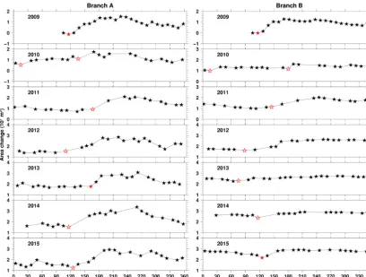
Further examination of the interannual variation indicates that the calving front exhibited different seasonal variations from year to year. First, even within a close distance of 10 km around the coastal area, branches A and B behaved asyn-chronously. For example, in 2010, Branch A began to re-treat in May, while Branch B started to rere-treat 1 month later (Figs. 6a and 7). Moreover, after 2012, Branch A’s front

un-derwent strong seasonal variation while Branch B’s front re-mained relatively stable (Fig. 6b). Second, the retreat timing of the glacier varied in different years. In Branch A, the front began to retreat around May in most years, while in 2011 and 2013 the retreat started in June. In 2010, both branches ex-perienced a sudden retreat from mid-January to early Febru-ary and then became stable. Third, the calving front variation became regular after 2012. In Branch A, the front stopped retreating in July of each year, and its position remained un-changed up to September to October. In Branch B, the front advanced in spring and retreated in early summer, while its position remained almost unchanged in other seasons (Figs. 5 and 7).

7 Discussion

7.1 Differences from the previous work

(9)

gener-Figure 7.Similar to Fig. 5 but showing the time series of calving front changes (in area changes) of our deep-learning-based results in different years. The red filled stars mark the dates when the glacier started to retreat. Red open stars mark starting dates that cannot be reliably determined due to data gaps (e.g., Branch A in 2011) and small variations (e.g., Branch B in 2013).

ate more accurate calving fronts. Without additional manual practices, our method is more transferable, particularly when applying to large areas with many glaciers. Below we discuss the technical differences in detail.

First, our study classifies the surface into two types (i.e., ice mélange and nonice mélange) to extract the calving front, while Mohajerani et al. (2019) used semantic segmentation to extract the front without classifying the surrounding sur-faces. Both strategies require postprocessing procedures. In our method, erroneous segmentation can cause small isolated polygons within the ice mélange or the nonice mélange re-gions. Yet, we can solve this problem by removing these small polygons in the postprocessing. The semantic segmen-tation used by Mohajerani et al. (2019) can be affected by icebergs, crevasses, etc. Nonetheless, the lowest-cost path search method could solve this problem (Mohajerani et al., 2019). Second, additional manual practices are needed in the work of Mohajerani et al. (2019). For instance, images of every single glacier in their work were adjusted by a certain angle to make all the glaciers flow in the same di-rection in the preprocessing. Third, we subdivide the im-ages into small patches, which allows us to utilize the ad-vantages of images with high resolution and various sizes.

Mohajerani et al. (2019) resampled images to a fixed size (240 pixels×152 pixels) with low spatial resolution (49.0 to 88.1 m); therefore the position accuracy is limited.

7.2 Calving front variation and bed elevation

In general, calving front variations are influenced by multiple factors, including floating or grounding conditions (McFad-den et al., 2011; Murray et al., 2015; Bondzio et al., 2017; Fried et al., 2018), interaction with the ocean (Holland et al., 2008; Howat et al., 2008; Motyka et al., 2011; Vieli and Nick, 2011; Straneo and Heimbach, 2013), ice mélange and sea ice conditions (Amundson et al., 2010; Moon et al., 2015; Cas-sotto et al., 2015), basal lubrication (Joughin et al., 2008b; Moon et al., 2014), and bed elevation (Joughin et al., 2008a, 2014; Kehrl et al., 2017; Bunce et al., 2018). Here we exam-ine the possible link between the observed variations of the calving fronts with bed elevation.

Bed elevation has a substantial influence on the glacier treat. In the first situation where the bed is flat, glacier re-treat decreases resisting force, which accelerates the glacier. The acceleration of the glacier can also thin the ice. Thin-ning reduces the effective pressure at the bed,N=Pi−Pw,

(10)

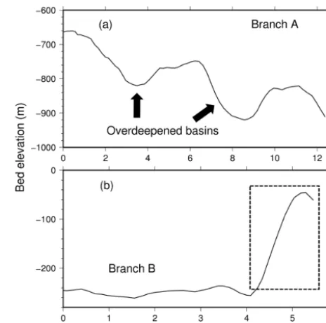
A decreased N reduces basal drag, causing stretching and faster flow and constituting positive feedback. In the second situation, as the glacier retreats into an overdeepened basin where the bed slopes down inland or is retrograde, the pos-itive feedback is reinforced, and the glacier becomes more unstable, for two reasons. First, ice thickness at the calving front increases as the retreat progresses, increasing driving stress. Second, because the calving front moves into deeper water, this retreat decreasesN further. In the third situation where the bed slopes inland–uphill, the glacier may stabi-lize, since retreating into shallower water increases N and decreases driving stress.

Previous studies also suggest that bed elevation has a sub-stantial influence on glacier calving front variations. Ex-amining the height above flotation of Branch A in Jakob-shavn, Joughin et al. (2014) suggested that retreating into an overdeepened basin where the bed slope is retrograde may lead to an unstable calving front retreat, and a bed sloping inland–uphill may stabilize the glacier. Other studies have also suggested that retreating into deeper water may acceler-ate the glacier, resulting in an unstable retreating (Howat et al., 2005, 2007; Nick et al., 2009; Catania et al., 2018).

In our study area, the bed elevation derived from BedMa-chine v3 (Morlighem et al., 2017) shows two overdeepened basins along the main channel of Branch A (Fig. 8a). During the period from 2009 to 2015, the calving front of Branch A retreated into the second overdeepened basin in August 2011 for the first time, which may have produced a faster rate of retreat. In July 2012, the glacier retreated to the bot-tom of the overdeepened basin and stopped retreating further (Movie S2). The inland–uphill bed slope behind the bottom of the overdeepened basin may have prevented the glacier from further retreating. In Branch B, after June 2012, the glacier retreated into a zone where the bed slopes uphill in-land (Fig. 8b, Movie S3). We suggest that retreating into this zone may have led to the more regular and stable behavior of Branch B after June 2012 (Fig. 5b).

7.3 Limitations of the current method

The current method is limited by high computational power requirement, and manual delineation largely controls its ac-curacy. First, the U-Net architecture requires relatively high GPU memory for large images. In our configuration, around 15 GB (gigabyte) of GPU memory is needed for training the network. Second, although splitting images with overlaps al-low us to apply the network to images with different sizes, the overlaps increase the training time. These two limitations can be overcome by hardware development. With more pow-erful GPUs in the future, we can increase the calculation ef-ficiency and lessen the training time. Third, the accuracy of this method relies on manual delineation as well as the in-formation richness of the training dataset (Goodfellow et al., 2016). If the training examples are not representative of the actual task or if the manual delineation in these examples is

Figure 8.Bed elevation profiles of two branches derived from Bed-Machine v3 (Morlighem et al., 2017). The profile locations are shown in Fig. 1a. The dashed box shows the zone where the bed slopes uphill inland.

of low quality or inconsistent, U-Net will either fail to train or will reproduce inconsistent results on new data. To further increase the accuracy and robustness of the network, more training examples are needed.

7.4 Prospects for future work

In the near future, we will include more training examples to minimize network error. In this study, the well-trained net-work is limited to a specific dataset, namely TSX images. However, it is feasible to apply the DCNN to multisensor remote sensing imagery, which has been proved by previ-ous studies (Nogueira et al., 2017; Lang et al., 2018). More-over, as long as the calving fronts are clear in the images, our method can also use images with light cloud cover and Landsat 7 images with scan line errors.

(11)

TerraSAR-X SAR images acquired from April 2009 to De-cember 2015. The small test error suggests that the accuracy of a well-trained network can be close to the human level. Our results reveal that the two branches of Jakobshavn Is-bræ behaved asynchronously. We suggest that bed elevation may have a major influence on the observed calving front variations. Our methodology can be applied to many other tidewater glaciers both in Greenland and elsewhere in the world using multitemporal and multisensor remote sensing imagery.

Code and data availability. The Greenland Ice Sheet CCI products

are available from http://products.esa-icesheets-cci.org (Markus and Joanna, 2017, last access: 8 October 2018). The bed elevation (BedMachine v3) is available from http://sites.uci.edu/morlighem/ dataproducts/bedmachine-greenland (Morlighem et al., 2017, last access: 17 October 2018). The code of the whole framework (Fig. 3) will be provided by Enze Zhang upon request. The network-delineated calving fronts obtained in this study are available from https://doi.org/10.1594/PANGAEA.897066 (Zhang et al., 2019).

Video supplement. Movie S1

(https://doi.org/10.1594/PANGAEA.897062, Zhang et al., 2019) shows the calving front positions from 16 April 2009 to 23 December. Movie S2 (https://doi.org/10.1594/PANGAEA.897080, Zhang et al., 2019) and Movie S3 (https://doi.org/10.1594/PANGAEA.897063, Zhang et al., 2019) show the calving front variation and the cross section between the calving front and the profile over branch A and branch B, respectively.

Supplement. The supplement related to this article is available

online at: https://doi.org/10.5194/tc-13-1729-2019-supplement.

Author contributions. EZ developed the code, performed the TSX

image analysis and calving front quantification, and wrote the manuscript. LL advised EZ and edited the manuscript. LH actively helped to develop the code.

Competing interests. The authors declare that they have no conflict

of interest.

Acknowledgements. We acknowledge the support of NVIDIA

Cor-poration, which donated the Quadro P5000 GPU used for this study. The TerraSAR-X SAR images were provided by the Deutsches Zen-trum für Luft- und Raumfahrt (DLR) (LAN1650, LAN1797, and COA3605). Our deep learning code is based on Jakeoung Koo’s

and suggestions, which significantly improved the quality of this paper.

Financial support. This research has been supported by the Hong

Kong Research Grants Council (grant no. CUHK24300414) and the CUHK Direct Grant for Research (grant no. 4053282).

Review statement. This paper was edited by Stef Lhermitte and

re-viewed by two anonymous referees.

References

Amundson, J. M., Fahnestock, M., Truffer, M., Brown, J., Lüthi, M. P., and Motyka, R. J.: Ice mélange dynamics and implications for terminus stability, Jakobshavn Isbræ, Greenland, J. Geophys. Res.-Earth, 115, F01005, https://doi.org/10.1029/2009JF001405, 2010.

Anantrasirichai, N., Biggs, J., Albino, F., Hill, P., and Bull, D.: Application of Machine Learning to Classification of Volcanic Deformation in Routinely Generated In-SAR Data, J. Geophys. Res.-Sol. Ea., 123, 6592–6606, https://doi.org/10.1029/2018JB015911, 2018.

Batista, G. E. A. P. A., Prati, R. C., and Monard, M. C.: Balancing Strategies and Class Overlapping, in: Lect. Notes Comput. Sc., 24–35, Springer Berlin Heidelberg, Berlin, Heidelberg, 2005. Bondzio, J. H.: Analysis of Recent Dynamic Changes of

Jakob-shavn Isbrae, West Greenland, Using a Thermomechanical Model, PhD thesis, University of Bremen, Germany, 175 pp., 2017.

Bondzio, J. H., Morlighem, M., Seroussi, H., Kleiner, T., Rückamp, M., Mouginot, J., Moon, T., Larour, E. Y., and Humbert, A.: The mechanisms behind Jakobshavn Isbræ’s acceleration and mass loss: A 3-D thermomechanical model study, Geophys. Res. Lett., 44, 6252–6260, https://doi.org/10.1002/2017GL073309, 2017. Bunce, C., Carr, J. R., Nienow, P. W., Ross, N., and Killick, R.: Ice

front change of marine-terminating outlet glaciers in northwest and southeast Greenland during the 21st century, J. Glaciol., 64, 523–535, https://doi.org/10.1017/jog.2018.44, 2018.

Cassotto, R., Fahnestock, M., Amundson, J. M., Truffer, M., and Joughin, I.: Seasonal and interannual varia-tions in ice melange and its impact on terminus stabil-ity, Jakobshavn Isbræ, Greenland, J. Glaciol., 61, 76–88, https://doi.org/10.3189/2015JoG13J235, 2015.

Catania, G. A., Stearns, L. A., Sutherland, D. A., Fried, M. J., Bartholomaus, T. C., Morlighem, M., Shroyer, E., and Nash, J.: Geometric Controls on Tidewater Glacier Retreat in Central Western Greenland, J. Geophys. Res.-Earth, 123, 2024–2038, https://doi.org/10.1029/2017JF004499, 2018.

(12)

Fried, M. J., Catania, G. A., Stearns, L. A., Sutherland, D. A., Bartholomaus, T. C., Shroyer, E., and Nash, J.: Reconciling Drivers of Seasonal Terminus Advance and Retreat at 13 Cen-tral West Greenland Tidewater Glaciers, J. Geophys. Res.-Earth, 123, 1590–1607, https://doi.org/10.1029/2018JF004628, 2018. Geng, J., Fan, J., Wang, H., Ma, X., Li, B., and Chen, F.:

High-Resolution SAR Image Classification via Deep Convolu-tional Autoencoders, IEEE Geosci. Remote S., 12, 2351–2355, https://doi.org/10.1109/LGRS.2015.2478256, 2015.

Goodfellow, I., Bengio, Y., and Courville, A.: Deep Learning, MIT Press, 2016.

Holland, D. M., Thomas, R. H., De Young, B., Ribergaard, M. H., and Lyberth, B.: Acceleration of Jakobshavn Isbrae triggered by warm subsurface ocean waters, Nat. Geosci., 1, 659–664, https://doi.org/10.1038/ngeo316, 2008.

Howat, I. M., Joughin, I., Tulaczyk, S., and Gogineni, S.: Rapid retreat and acceleration of Helheim Glacier, east Greenland, Geophys. Res. Lett., 32, L22502, https://doi.org/10.1029/2005GL024737, 2005.

Howat, I. M., Joughin, I., and Scambos, T. A.: Rapid Changes in Ice Discharge from Greenland Outlet Glaciers, Science, 315, 1559– 1561, https://doi.org/10.1126/science.1138478, 2007.

Howat, I. M., Joughin, I., Fahnestock, M., Smith, B. E., and Scambos, T. A.: Synchronous retreat and acceleration of southeast Greenland outlet glaciers 2000–06: ice dy-namics and coupling to climate, J. Glaciol., 54, 646–660, https://doi.org/10.3189/002214308786570908, 2008.

Howat, I. M., Ahn, Y., Joughin, I., van den Broeke, M. R., Lenaerts, J. T. M., and Smith, B.: Mass balance of Greenland’s three largest outlet glaciers, 2000–2010, Geophys. Res. Lett., 38, L12501, https://doi.org/10.1029/2011GL047565, 2011.

Huang, Z., Pan, Z., and Lei, B.: Transfer Learning with Deep Convolutional Neural Network for SAR Target Classifica-tion with Limited Labeled Data, Remote Sens.-Basel, 9, 907, https://doi.org/10.3390/rs9090907, 2017.

Joughin, I., Abdalati, W., and Fahnestock, M.: Large fluctuations in speed on Greenland’s Jakobshavn Isbrae glacier, Nature, 432, 608–610, https://doi.org/10.1038/nature03130, 2004.

Joughin, I., Howat, I., Alley, R. B., Ekstrom, G., Fahnestock, M., Moon, T., Nettles, M., Truffer, M., and Tsai, V. C.: Ice-front variation and tidewater behavior on Helheim and Kangerd-lugssuaq Glaciers, Greenland, J. Geophys. Res.-Earth, 113, F01004, https://doi.org/10.1029/2007JF000837, 2008a. Joughin, I., Das, S. B., King, M. A., Smith, B. E., Howat,

I. M., and Moon, T.: Seasonal Speedup Along the Western Flank of the Greenland Ice Sheet, Science, 320, 781–783, https://doi.org/10.1126/science.1153288, 2008b.

Joughin, I., Howat, I. M., Fahnestock, M., Smith, B., Krabill, W., Alley, R. B., Stern, H., and Truffer, M.: Continued evolution of Jakobshavn Isbrae following its rapid speedup, J. Geophys. Res.-Earth, 113, F04006, https://doi.org/10.1029/2008JF001023, 2008c.

Joughin, I., Smith, B. E., Howat, I. M., Floricioiu, D., Alley, R. B., Truffer, M., and Fahnestock, M.: Seasonal to decadal scale vari-ations in the surface velocity of Jakobshavn Isbrae, Greenland: Observation and model-based analysis, J. Geophys. Res.-Earth, 117, F02030, https://doi.org/10.1029/2011JF002110, 2012. Joughin, I., Smith, B. E., Shean, D. E., and Floricioiu, D.: Brief

Communication: Further summer speedup of Jakobshavn Isbræ,

The Cryosphere, 8, 209–214, https://doi.org/10.5194/tc-8-209-2014, 2014.

Kehrl, L. M., Joughin, I., Shean, D. E., Floricioiu, D., and Krieger, L.: Seasonal and interannual variabilities in terminus position, glacier velocity, and surface elevation at Helheim and Kanger-lussuaq Glaciers from 2008 to 2016, J. Geophys. Res.-Earth, 122, 1635–1652, https://doi.org/10.1002/2016JF004133, 2017. King, M. D., Howat, I. M., Jeong, S., Noh, M. J., Wouters, B., Noël,

B., and van den Broeke, M. R.: Seasonal to decadal variability in ice discharge from the Greenland Ice Sheet, The Cryosphere, 12, 3813–3825, https://doi.org/10.5194/tc-12-3813-2018, 2018. Kingma, D. P. and Ba, J.: Adam: A Method for Stochastic

Opti-mization, ICLR, available at: http://arxiv.org/abs/1412.6980 (last access: 17 January 2019), 2015.

Lang, G., Tian, T., Xiao, S., and Hang, L.: Fusion of shallow and deep features for classification of high-resolution remote sensing images, in: MIPPR 2017: Multispectral Image Ac-quisition, Processing, and Analysis, vol. 10607, p. 106070O, https://doi.org/10.1117/12.2284777, 2018.

LeCun, Y., Bengio, Y., and Hinton, G.: Deep learning, Nature, 521, 436–444, https://doi.org/10.1038/nature14539, 2015.

Luckman, A. and Murray, T.: Seasonal variation in velocity before retreat of Jakobshavn Isbræ, Greenland, Geophys. Res. Lett., 32, L08501, https://doi.org/10.1029/2005GL022519, 2005. Maas, A. L., Hannun, A. Y., and Ng, A. Y.: Rectifier nonlinearities

improve neural network acoustic models, in: ICML Workshop on Deep Learning for Audio, Speech and Language Processing, 2013.

McFadden, E. M., Howat, I. M., Joughin, I., Smith, B. E., and Ahn, Y.: Changes in the dynamics of marine terminating outlet glaciers in west Greenland (2000–2009), J. Geophys. Res.-Earth, 116, F02022, https://doi.org/10.1029/2010JF001757, 2011.

Meier, M. F. and Post, A.: Fast tidewater glaciers, J. Geophys. Res.-Sol. Ea., 92, 9051–9058, https://doi.org/10.1029/JB092iB09p09051, 1987.

Mohajerani, Y., Wood, M., Velicogna, I., and Rignot, E.: Detection of Glacier Calving Margins with Convolutional Neural Networks: A Case Study, Remote Sens., 11, 74, https://doi.org/10.3390/rs11010074, 2019.

Moon, T. and Joughin, I.: Changes in ice front position on Green-land’s outlet glaciers from 1992 to 2007, J. Geophys. Res.-Earth, 113, F02022, https://doi.org/10.1029/2007JF000927, 2008. Moon, T., Joughin, I., Smith, B., van den Broeke, M. R., van de

Berg, W. J., Noël, B., and Usher, M.: Distinct patterns of seasonal Greenland glacier velocity, Geophys. Res. Lett., 41, 7209–7216, https://doi.org/10.1002/2014GL061836, 2014.

Moon, T., Joughin, I., and Smith, B.: Seasonal to multiyear variabil-ity of glacier surface velocvariabil-ity, terminus position, and sea ice/ice mélange in northwest Greenland, J. Geophys. Res.-Earth, 120, 818–833, https://doi.org/10.1002/2015JF003494, 2015. Morlighem, M., Williams, C. N., Rignot, E., An, L., Arndt, J. E.,

(13)

Rysgaard, S., and Howat, I.: Submarine melting of the 1985 Jakobshavn Isbræ floating tongue and the triggering of the current retreat, J. Geophys. Res.-Earth, 116, F01007, https://doi.org/10.1029/2009JF001632, 2011.

Murray, T., Selmes, N., James, T. D., Edwards, S., Martin, I., O’Farrell, T., Aspey, R., Rutt, I., Nettles, M., and Baugé, T.: Dy-namics of glacier calving at the ungrounded margin of Helheim Glacier, southeast Greenland, J. Geophys. Res.-Earth, 120, 964– 982, https://doi.org/10.1002/2015JF003531, 2015.

Nick, F. M., Vieli, A., Howat, I. M., and Joughin, I.: Large-scale changes in Greenland outlet glacier dynam-ics triggered at the terminus, Nat. Geosci., 2, 110–114, https://doi.org/10.1038/ngeo394, 2009.

Nogueira, K., Penatti, O. A., and dos Santos, J. A.: Towards better exploiting convolutional neural networks for remote sensing scene classification, Pattern Recogn., 61, 539–556, https://doi.org/10.1016/j.patcog.2016.07.001, 2017.

Ronneberger, O., Fischer, P., and Brox, T.: U-Net: Convolutional Networks for Biomedical Image Segmentation, in: Lect. Notes Comput. Sc., edited by: Navab, N., Hornegger, J., Wells, W. M., and Frangi, A. F., Springer International Publishing, Cham, 234– 241, 2015.

Rosenau, R., Schwalbe, E., Maas, H.-G., Baessler, M., and Dietrich, R.: Grounding line migration and high-resolution calving dy-namics of Jakobshavn Isbræ, West Greenland, J. Geophys. Res.-Earth, 118, 382–395, https://doi.org/10.1029/2012JF002515, 2013.

Roth, A., Huber, M., and Kosmann, D.: Geocoding of TerraSAR-X data, Proc. Int. 20th ISPRS Congr., 840–844, 2004.

Seale, A., Christoffersen, P., Mugford, R. I., and O’Leary, M.: Ocean forcing of the Greenland Ice Sheet: Calving fronts and patterns of retreat identified by automatic satellite monitoring of eastern outlet glaciers, J. Geophys. Res.-Earth, 116, F03013, https://doi.org/10.1038/ngeo765, 2011.

shavn Glacier, west Greenland: 30 years of space-borne observations, Geophys. Res. Lett., 25, F03013, https://doi.org/10.1029/2010JF001847, 1998.

Straneo, F. and Heimbach, P.: North Atlantic warming and the retreat of Greenland’s outlet glaciers, Nature, 504, 36–43, https://doi.org/10.1038/nature12854, 2013.

Sun, Y., Wang, X., and Tang, X.: Deep learning face representation from predicting 10,000 classes, in: Proceedings of the IEEE con-ference on computer vision and pattern recognition, 1891–1898, 2014.

Thomas, R. H.: Force-perturbation analysis of recent thinning and acceleration of Jakobshavn Isbræ, Greenland, J. Glaciol., 50, 57– 66, https://doi.org/10.3189/172756504781830321, 2004. Vieli, A. and Nick, F. M.: Understanding and Modelling

Rapid Dynamic Changes of Tidewater Outlet Glaciers: Issues and Implications, Surv. Geophys., 32, 437–458, https://doi.org/10.1007/s10712-011-9132-4, 2011.

Xie, S., Dixon, T. H., Voytenko, D., Holland, D. M., Hol-land, D., and Zheng, T.: Precursor motion to iceberg calv-ing at Jakobshavn Isbræ, Greenland, observed with ter-restrial radar interferometry, J. Glaciol., 62, 1134–1142, https://doi.org/10.1017/jog.2016.104, 2016.

Zhang, E., Liu, L., Huang, L.: Calving front and the comparison between its variations and bed elevation in Jakobshavn Isbræ, https://doi.pangaea.de/10.1594/PANGAEA.897066, 2019. Zhang, F., Du, B., and Zhang, L.: Saliency-Guided