https://doi.org/10.5194/tc-13-557-2019
© Author(s) 2019. This work is distributed under the Creative Commons Attribution 4.0 License.
Mapping pan-Arctic landfast sea ice stability using
Sentinel-1 interferometry
Dyre O. Dammann1, Leif E. B. Eriksson1, Andrew R. Mahoney2, Hajo Eicken3, and Franz J. Meyer2
1Department of Space, Earth and Environment, Chalmers University of Technology, Gothenburg, 41296, Sweden 2Geophysical institute, University of Alaska Fairbanks, Fairbanks, 99775, USA
3International Arctic Research Center, University of Alaska Fairbanks, Fairbanks, 99775, USA
Correspondence:Dyre O. Dammann ([email protected]) Received: 22 June 2018 – Discussion started: 11 July 2018
Revised: 23 December 2018 – Accepted: 19 January 2019 – Published: 18 February 2019
Abstract. Arctic landfast sea ice has undergone substantial changes in recent decades, affecting ice stability and includ-ing potential impacts on ice travel by coastal populations and on industry ice roads. We present a novel approach for evaluating landfast sea ice stability on a pan-Arctic scale us-ing Synthetic Aperture Radar Interferometry (InSAR). Us-ing Sentinel-1 images from sprUs-ing 2017, we discriminate be-tween bottomfast, stabilized, and nonstabilized landfast ice over the main marginal seas of the Arctic Ocean (Beau-fort, Chukchi, East Siberian, Laptev, and Kara seas). This approach draws on the evaluation of relative changes in in-terferometric fringe patterns. This first comprehensive as-sessment of Arctic bottomfast sea ice extent has revealed that most of the bottomfast sea ice is situated around river mouths and coastal shallows. The Laptev and East Siberian seas dominate the aerial extent, covering roughly 4100 and 5100 km2, respectively. These seas also contain the largest extent of stabilized and nonstabilized landfast ice, but are subject to the largest uncertainties surrounding the mapping scheme. Even so, we demonstrate the potential for using In-SAR for assessing the stability of landfast ice in several key regions around the Arctic, providing a new understanding of how stability may vary between regions. InSAR-derived sta-bility may serve for strategic planning and tactical decision support for different uses of coastal ice. In a case study of the Nares Strait, we demonstrate that interferograms may reveal early-warning signals for the breakup of stationary sea ice.
1 Introduction
1.1 Landfast sea ice stability and stakeholder dependence
Sea ice is an important component of Arctic ecosystems and provides important functions as a climate regulator (Screen and Simmonds, 2010), habitat for marine biota (Thomas, 2017), and a platform for coastal populations (Krupnik et al., 2010). During the last century, an expansion of trans-portation and resource extraction have led to increased hu-man presence in the Arctic and further diversification of ice use (Eicken et al., 2009). The recent retreat of sea ice ob-served over the past several decades (Stroeve et al., 2012; Comiso and Hall, 2014; Meier et al., 2014) has already resulted in widespread consequences for ice users (ACIA, 2004; Aporta and Higgs, 2005; Fienup-Riordan and Rear-den, 2010; Orviku et al., 2011; Druckenmiller et al., 2013), as well as increasing hazards (Ford et al., 2008; Eicken and Mahoney, 2015). At the same time, the related increased ac-cessibility to Arctic waters (Stephenson et al., 2011) is lead-ing to more ship traffic and resource exploration (Lovecraft and Eicken, 2011; Eguíluz et al., 2016). It is further recog-nized that sea ice conditions for future Arctic marine opera-tions will be challenging, and will require substantial mon-itoring and improved observations (Arctic Council, 2009). This improvement will require observations on local and re-gional scales in order to provide an assessment of environ-mental hazards and effective emergency responses (Eicken et al., 2011).
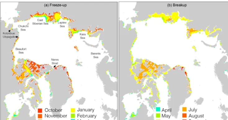
Figure 1. (a)October–March (freeze-up) and(b)April–September (breakup) monthly mean landfast sea ice extent (1976–2007), derived from sea ice charts based on optical instruments and SAR. The data for this figure were obtained from the National Snow and Ice Data Center (Yu et al., 2014).
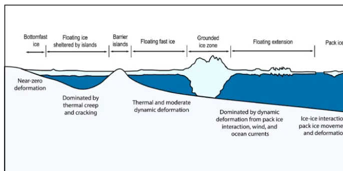
Arctic coastlines roughly between November and June, de-pending on location (Fig. 1; Yu et al., 2014). Sections of land-fast ice, often from several kilometers to hundreds of kilome-ters wide, are held in place by grounded ridges, islands, or coastline morphology, such as embayments or fjords. Sim-ilar to drifting pack ice, landfast ice has declined signifi-cantly during the last few decades, particularly in terms of delayed freeze-up in the Beaufort (Mahoney et al., 2014) and Laptev (Selyuzhenok et al., 2015) seas, as well as to a significantly reduced extent in the Chukchi Sea (Mahoney et al., 2014). Later freeze-up critically impacts stakeholders through reduced stability of landfast ice in response to fewer grounded ridges capable of withstanding wind, ocean, or ice forcing (Dammann, 2017). Previous research suggests that landfast ice stability can be expressed in terms of combined frictional resistance provided by relevant grounding or at-tachment points (e.g., islands and grounded ridges; Mahoney et al., 2007; Druckenmiller, 2011). Although landfast ice is stationary, it deforms at the centimeter to meter scale, on timescales of days to months due to forcing from wind, cur-rents, and drifting ice (Dammann et al., 2016). Its stability in part determines the rate at which the ice deforms, and ulti-mately, the severity of breakout events or magnitude of struc-tural defects. We suggest that landfast sea ice can be further categorized into three regimes, defined through their respec-tive stabilities: (1) bottomfast ice, (2) floating ice enclosed in lagoons or fjords, or sheltered by point features such as grounded ridges or islands, and (3) floating ice extensions (Table 1). A typical landfast ice regime is illustrated in Fig. 2, where the stability of the landfast ice area decreases from the coast toward the open ocean (Dammann et al., 2016).
Bottomfast sea ice can grow laterally to kilometer scale during winter, depending on local bathymetry (Solomon et
al., 2008; Stevens et al., 2010). This bottomfast ice allows for heat loss from the seafloor and is therefore an integral part of aggregating and maintaining subsea permafrost (Solomon et al., 2008; Stevens et al., 2008, 2010; Stevens, 2011), as well as controlling coastal stability and morphology (Are and Reimnitz, 2000; Eicken et al., 2005). Bottomfast ice is also relevant for fish, as it reduces habitable shallow waters dur-ing winter (Hirose et al., 2008), and for on-ice operations, as it can support a much larger load than floating ice. High to moderately stable landfast ice is of relevance to industrial (Potter et al., 1981) and subsistence ice use (Druckenmiller et al., 2013), as well as for habitats (Tibbles et al., 2018). Ringed seals, for instance, are dependent on stable land-fast ice for denning (Smith, 1980). Low-stability ice is po-tentially relevant for ocean-based operations, such as ship-ping through trans-Arctic passages close to the coast, where patches of landfast ice occasionally break off and drift into nearby shipping lanes, potentially causing hazards. Even ar-eas hundreds of kilometers from landfast ice can be impacted through the failure of ice arches.
typ-Figure 2.Conceptual scheme of landfast sea ice, where different regimes possess different levels of stability.
ically collapse in July–August (Kwok, 2005). Conversely, their breakup can lead to the advection of large amounts of thick multiyear ice into high-traffic shipping routes (Barber et al., 2018), creating a well-known hazard (Bailey, 1957; Wilson et al., 2004; Howell et al., 2013). Recent and ongo-ing sea ice decline is leadongo-ing to an increasongo-ing presence of thinner ice in the Canadian Archipelago (Haas and Howell, 2015), and weaker ice due to warmer temperatures (Melling, 2002) may lead to earlier breaching of ice arches. This could result in a larger amount of advected ice with potentially longer travel paths, increasing the severity of such events (Melling, 2002; Barber et al., 2018). One location of partic-ular interest is the Nares Strait, situated between Greenland and Ellesmere Island, featuring a seasonal ice arch (Kwok, 2005; Kwok et al., 2010) with important implications for the multiyear ice budget of the Arctic Ocean (Kwok et al., 2010). This stability is also relevant for destinational cargo shipping in the Arctic, as less stable, thinner ice is easier to break through, resulting in opportunities for docking in areas of landfast ice. For navigating through landfast ice, stabiliza-tion through ridging is also important to identify, as ridges can be problematic to navigate and are often associated with hazards (Hui et al., 2017).
1.2 Remote sensing of landfast ice stability
Satellite remote sensing is an important tool for measuring ice conditions in the Arctic, including the mapping of land-fast ice (Muckenhuber and Sandven, 2017). Optical and ther-mal satellite data, such as from the Advanced Very High Res-olution Radiometer (AVHRR), were used to produce opera-tional ice charts until the early 1990s, when SAR was in-troduced into the charting production (Yu et al., 2014) as a superior data set, thanks to its independence from light and weather conditions and its higher (∼100 m) resolution – both advantageous to stakeholders (Eicken et al., 2011). Different techniques exist to map the boundaries of
land-fast sea ice, typically derived by evaluating unchanged sec-tions of ice between consecutive SAR backscatter scenes (Johannessen et al., 2006; Giles et al., 2008; Mahoney et al., 2014). In addition to its use in the mapping of landfast ice, SAR backscatter can also discriminate between multi-year and first-multi-year ice (Onstott, 1992) and identify different roughness regimes (Dammann et al., 2017). SAR has also been used to estimate the advection of ice through straits in the Canadian Archipelago (Melling, 2002; Kwok, 2006; Howell et al., 2013). However, SAR backscatter typically does not give information pertaining to the stability of land-fast ice or temporarily stabilized pack ice, since the internal movement of the landfast ice is too small (mm day−1) to be identified with change detection.
These studies have demonstrated (1) the potential of In-SAR as a tool for assessing landfast ice dynamics and stabil-ity through local case studies and (2) its utilstabil-ity as a planning tool for on-ice operations (Dammann et al., 2018a, b). They have also laid the foundation for applying InSAR on a larger scale, potentially as a means for generating operational infor-mation products and evaluating long-term trends. The cover-age and access to InSAR-compatible SAR scenes has been an obstacle in the past, but has improved significantly since the launch of Sentinel-1 (the suitability of Sentinel-1 for au-tomatic SAR processing has been shown, e.g., in Meyer et al., 2015). In this study, we explore InSAR as a tool for pro-viding pan-Arctic information on ice stability, which is rel-evant to subsea permafrost, biological habitats, and sea ice use. The goal of this work is to determine Sentinel-1 in-terferometric data availability along substantial parts of the circumpolar coastlines and to explore their applicability for consistently mapping landfast sea ice stability zones in dif-ferent geographic regions. We further explore the limitations of the technology and possible applications.
2 Data and methods 2.1 InSAR principles
The interferometric phase may be related to lateral (e.g., thermal contraction or displacement due to compressional or shear forces) or vertical (e.g., through buckling or tidal displacement) sea ice motion that occurs in between the ac-quisition times for the two SAR images. A phase signature can sometimes also be attributed to factors not related to sur-face motion, such as atmospheric phase delay. Of the phase change attributed to motion, only displacement in line-of-sight direction (1rLOS) results in a phase change 18disp,
according to 18disp=4π 1rLOS/λ. The observed phase is
measured within the wrapped interval of [0;2π[. The inter-ferogram is a series of fringes representing the projection of the true three-dimensional ice motion onto the line-of-sight vector. The orientation of fringes can be used to interpret the direction of the three-dimensional motion field, and fringe spacing is an indicator of the deformation rate. The interpre-tation of observed fringe patterns is, however, not straight-forward, and it typically requires the use of an inverse model (Dammann et al., 2016). The interferometric phase values will only be useful if scattering elements remain largely un-changed throughout the time interval bracketed by the im-age pairs used in processing. InSAR phase stability, referred to as InSAR coherence, depends largely on topography cou-pled with a perpendicular baseline, as well as the temporal stability of the scatterers on the ground surface. Coherence ranges between 0 (pure noise) and 1 (no noise), and serves as a measure of the quality of the interferogram. Coherence is generally high if scatterers remain unchanged and low if
there is significant change in the scattering medium (Meyer et al., 2011).
2.2 Sentinel-1 data
This study uses Sentinel-1, a constellation of two C-band SAR systems (Sentinel-1A and B) in operation since 2014 and 2016, with a repeat-pass interval of 6 to 12 days, depend-ing on whether both or just one of the satellites acquire data. Thanks to a free-and-open data policy and large spatial cov-erage, we obtained Sentinel-1 acquisitions for five marginal seas of the Arctic Ocean, enabling mapping of landfast sea ice on a pan-Arctic scale. All images used were captured in interferometric wideswath (IW) mode, with a single-look resolution of roughly 3 m×22 m in slant range and azimuth, and a∼250 km swath width. Images were acquired almost exclusively between March and May 2017 (see Supplement for full list of images used). We acquired over 100 SAR im-ages, covering nearly the entire continental coastlines of the Beaufort, Chukchi, East Siberian, Laptev, and Kara seas. To reduce computational costs, we omitted Greenland, some is-land groups, and the Canadian Archipelago, which are char-acterized by extensive coastline lengths. In this work, we fo-cused on the Alaska and Russian marginal seas of the Arctic Ocean. These coastlines have high economic significance for the shipping and natural resource industries, and also feature dynamically diverse ice regimes. Large areas of bottomfast ice are expected in these regions. Except for one approxi-mately 50 km long section of coast in the Kara Sea and the eastern Laptev Sea, multiple InSAR compatible pairs were available for the specified time frame. This allowed us to se-lect interferograms centered around the end of April, when most Arctic landfast ice is at its maximum extent and thick-ness.
In addition to images obtained for the large-scale map-ping of stability zones, a series of six consecutive image pairs were acquired covering the Nares Strait and the breakup of an ice arch during spring 2017. This image sequence featured a 6-day temporal baseline covering a time span of 36 days.
2.3 Data processing
However, coherence loss was evident in some areas – in par-ticular in the Chukchi Sea, such as in the Kotzebue Sound. This was likely predominately due to surface melt, as air temperature reached above freezing between SAR acquisi-tions. Other possible contributing reasons for coherence loss in this region could include ice motion, subsurface ice thin-ning from river runoff, and low signal-to-noise ratio. Signif-icant decorrelation can also occur in late spring, as the onset of melt causes substantial changes in the scattering medium. In this work, we obtained images as close to late April as pos-sible. This time frame was found to be ideal for our purpose, as ice thickness is near its maximum, leading to maximum stability and minimizing impacts from the onset of melt. To ensure a realistic representation of an operationally produced synoptic, contiguous pan-Arctic interferogram, we did not at-tempt to derive alternative interferograms (i.e., different time periods) in cases of low coherence.
All backscatter images and interferograms in this work were produced using a standard Sentinel-1 workflow in Gamma software (Werner et al., 2000). The IW images ini-tially consist of independent bursts and swaths, which we combined to utilize the full extent of the acquisition. We fur-ther coregistered pairs of acquisitions to ensure images cover exactly the same area with subpixel accuracy. Images were then multilooked, averaging 10 pixels in range and 2 pix-els in azimuth, resulting in reduced speckle and a final pixel spacing of roughly 23×28 m. Next, spectral filtering was performed to ensure both images comprise the same spec-tral range, reducing phase noise in the final interferogram. The interferometric phase was calculated for each pixel of the coregistered and filtered images. Furthermore, the ex-pected phase ramp in cross-track direction from a station-ary flat earth surface was removed. The phase noise of the final interferogram was reduced using an adaptive phase fil-ter (Goldstein and Werner, 1998). The result was 52 infil-ter- inter-ferograms, covering almost the entire coastline between the Canadian Archipelago and the Barents Sea.
2.4 Mapping landfast ice stability zones
In this work, we evaluated relative ice stability based on fringe spacings within individual interferograms. This al-lowed us to identify variations within an area imaged under largely the same conditions (e.g., close to the same wind and ocean forcing). Trends from higher to lower fringe density will likely correspond to increasing ice stability. Therefore, interferograms can provide information related to the spatial variations in stability. Meyer et al. (2011) demonstrated that interferometry can be used to map the landfast ice based on a coherent phase response. Their work also suggested that fringe patterns are significantly impacted by grounded ridges and reduced fringe density. Dammann et al. (2018c) further showed that bottomfast ice can be mapped based on a near-zero phase change where ice is frozen to the seafloor. We built on this work by suggesting that InSAR can be used to
map three different zones of relative stability: bottomfast ice, stabilized ice, and nonstabilized ice (Table 1). These three zones are subjectively and manually mapped without the use of specific threshold values.
Bottomfast ice is identified with near-zero phase change in the interferogram. It can often be distinguished from adja-cent floating ice commonly featuring a nonzero phase change or low coherence (Fig. 3a). The shoreward boundary of bot-tomfast ice is difficult to obtain from the interferogram alone, since the phase signatures over bottomfast ice and low-lying coastal areas are similar. The use of the landmask (Wessel and Smith, 1996) is not ideal, since subtle coastal features such as sediment bars are often not captured. We therefore delineated the coastline (i.e., shoreward boundary of bottom-fast ice) using the backscatter signature in a composite im-age with backscatter and phase (Fig. 3b). Plotting bottomfast ice with the landmask can thus give the wrongful appearance that (1) areas of near-zero phase should have been mapped as bottomfast and (2) bottomfast ice appears in sporadic areas along the coast separated by floating ice.
We could often identify stabilized ice by a stark fringe dis-continuity between different fringe densities (Fig. 3c). How-ever, in some regions, changes in stability are more grad-ual between zones (Figs. 6c and 7c). Mapping of such re-gions are therefore more subjective and possibly less exact. In cases lacking stark fringe discontinuities, stabilized ice is also mapped in regions featuring a very slight phase response with no clear fringe patterns (Fig. 3d).
Nonstabilized ice is identified as landfast ice (i.e., areas featuring relatively high interferometric coherence) other-wise not marked as bottomfast or stabilized ice. Nonstabi-lized ice commonly features clear fringe patterns (Fig. 3e).
2.5 Validation areas and data
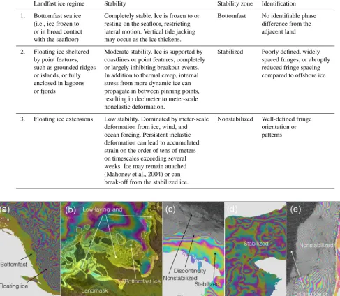
Table 1.Landfast sea ice stability regimes and assigned stability zones identified using InSAR.
Landfast ice regime Stability Stability zone Identification
1. Bottomfast sea ice Completely stable. Ice is frozen to or Bottomfast No identifiable phase (i.e., ice frozen to resting on the seafloor, restricting difference from the or in broad contact lateral motion. Vertical tide jacking adjacent land with the seafloor) may occur as the ice thickens.
2. Floating ice sheltered Moderate stability. Ice is supported by Stabilized Poorly defined, widely by point features, coastlines or point features, completely spaced fringes, or abruptly such as grounded ridges or largely inhibiting breakout events. reduced fringe spacing or islands, or fully In addition to thermal creep, internal compared to offshore ice enclosed in lagoons stress from more dynamic ice can
or fjords propagate in between pinning points, resulting in decimeter to meter-scale nonelastic deformation.
3. Floating ice extensions Low stability. Dominated by meter-scale Nonstabilized Well-defined fringe
deformation from ice, wind, and orientation or
ocean forcing. Persistent inelastic patterns deformation can lead to accumulated
strain on the order of tens of meters on timescales exceeding several weeks. Ice may remain attached (Mahoney et al., 2004) or can break-off from the stabilized ice.
Figure 3. (a)Example of interferometric phase response over bottomfast ice.(b)Phase/backscatter composite near a delta. This example exhibits a poor match between the landmask (transparent black shading) and low-lying coastal areas. Here, bottomfast ice (white outline) had to be mapped against the coastline, as identified in the backscatter data.(c)Example of stabilized ice as identified based on a phase discontinuity.(d)Example of stabilized ice as identified by low fringe density and nonconsistent fringe patterns.(e)Example of nonstabilized ice as identified by high fringe density. Land is masked out in light gray in panels(a, c, d, e).
3 Results
3.1 Evaluating landfast ice stability zones
We constructed a series of Sentinel-1 interferograms along the coastlines of five marginal seas in the Arctic Ocean dur-ing 2017: the Beaufort, Chukchi, East Siberian, Laptev, and Kara seas. As seen in the interferograms (Figs. 4–8), landfast sea ice varies substantially between the seas in terms of the extent and interferometric fringe density.
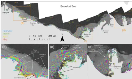
pat-Figure 4. (a)Sentinel-1 interferograms derived from image pairs acquired over the Beaufort Sea between March and May 2017. Numbers on images represent date ranges. The colors blue, green, yellow, and red signify the months of February–May.(b, c, d)Three enlarged areas identified in(a)are further discussed in the text.
tern surrounding grounded ridges. This is because grounded ridges result in a shoreward increase in stability that does not extend to areas immediately to the side of the ridges (the alongshore direction). Examples of likely grounding points are indicated with white arrows in Fig. 4b, and similar pat-terns are also apparent near the Mackenzie Delta (Fig. 4c). The landfast ice in the eastern part of the Beaufort Sea also consists of large areas of stabilized ice. Here, the landfast ice is noticeably sheltered by land features, resulting in lower-density fringes (Fig. 4d).
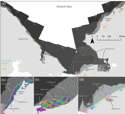
Landfast sea ice in the Chukchi Sea is generally less ex-tensive than in the Beaufort Sea, particularly along the Rus-sian coast (Fig. 5a). Bottomfast ice in the Chukchi is con-strained mostly to lagoons. Some of these lagoons, such as the Kasegaluk, consist almost exclusively of bottomfast ice (Fig. 5b). Only a few areas of landfast ice appear to be sta-bilized, including the northern coast of Alaska near Peard Bay (Fig. 5c) and the southern Chukchi Sea near Shishmaref (Fig. 5d). The Chukchi Sea consists predominantly of non-stabilized ice, with the most extensive region of landfast ice situated off the shore of the village of Shishmaref (Fig. 5d). The Chukchi Sea features coherence loss in several regions such as the Kotzebue Sound (Fig. 5a).
The landfast ice in the East Siberian Sea is more extensive than in the Chukchi and Beaufort seas and can extend over 100 km from the shore (Fig. 6a). Bottomfast ice is also more extensive than in the Beaufort and Chukchi seas. The bot-tomfast ice in the East Siberian Sea follows several sections
of coastline even tens of kilometers away from major rivers, though most of the bottomfast ice is situated near the Kolyma and Indigirka deltas (Fig. 6b). In contrast to the Beaufort and Chukchi seas, stabilized ice extends several tens of kilome-ters offshore without being sheltered by coastline morphol-ogy or islands (Fig. 6c). These large areas also lack clear indications of the presence of grounded ridges (Fig. 6d).
Figure 5. (a)Sentinel-1 interferograms derived from image pairs acquired over the Chukchi Sea between March and May 2017. Numbers on images represent date ranges. The colors blue, green, yellow, and red signify the months of February–May.(b, c, d)Three enlarged areas identified in(a)are further discussed in the text.
Landfast ice in the Kara Sea features a much smaller ice extent than the other Russian seas (Fig. 8a). Bottomfast ice is also much less prevalent and largely situated near the Pyasina River (Fig. 8b). The landfast ice extends tens of kilometers from shore, predominately in areas supported by offshore is-lands and archipelagos (Fig. 8c, d). In these archipelagos, the ice confined by islands is largely stabilized (Fig. 8c).
Interferograms have enabled the mapping of landfast ice stability zones based on subjective interpretations of inter-ferometric fringes (Fig. 9). The resulting stability map allows for a large-scale comparison and analysis of bottomfast, sta-bilized, and nonstabilized landfast ice, within and between the different seas. For this comparison, we have calculated the area of each stability zone (Table 2). However, it is im-portant to note these area calculations are not complete, as the analysis omitted some island groups and included some data gaps.
Most areas with extensive bottomfast ice reaching several kilometers from shore are located either in the vicinity of river deltas or within lagoons. The East Siberian Sea and its three large river systems (the Indigirka, Bogdashkina, and Kolyma rivers) contain the most bottomfast ice of the regions considered here. The Laptev Sea also contains a large area of bottomfast sea ice. Together, the Laptev and East Siberian seas contain over half (∼57 %) of the total areal extent of bottomfast ice calculated, while the Chukchi Sea features the lowest extent of bottomfast ice of the regions considered here. Bottomfast ice is predominately situated in lagoons.
Figure 6. (a) Sentinel-1 interferograms derived from image pairs acquired over the East Siberian Sea between March and May, 2017. Numbers on images represent date ranges. The colors blue, green, yellow, and red signify the months of February–May.(b, c, d)Three enlarged areas identified in(a)are further discussed in the text.
Table 2.Approximate area coverage of landfast ice (in thousand km2).
Area Bottomfast Stabilized Nonstabilized Total area of Area fraction: landfast ice nonstabilized/stabilized
Beaufort Sea 2.5 35 29 67 0.83
Chukchi Sea 1.8 4.6 25 31 5.43
East Siberian Sea 5.1 45 80 130 1.78
Laptev Sea 4.1 74 127 205 1.72
Kara Sea 2.6 16 37 56 2.3
The bottomfast ice zone is constrained between its outer extent (interpreted from the phase) and the coast (as interpreted from the backscatter scenes). The stabilized zone is constrained between its outer extent (as interpreted from the phase) and the bottomfast ice or the landmask (Wessel and Smith, 1996). The nonstabilized ice is constrained between the outer extent of nonzero coherence and the bottomfast ice, stabilized ice, or the landmask.
delineated here, the Beaufort Sea is the only sea that features more stabilized ice than nonstabilized ice. This is likely at-tributed to the large grounded sections, as well as areas shel-tered by coastal morphology. The Laptev Sea also features large areas confined by coastlines. However, in the Laptev sea, these regions also commonly feature nonstabilized ice. Meanwhile a large part of the landfast ice in the Kara Sea is mapped as stabilized, largely due to the fraction of landfast ice situated between islands and archipelagos. With a rela-tively narrow landfast ice extent compared to other seas and the absence of regions of sheltered ice, the Chukchi Sea con-tains the lowest total extent of stabilized ice.
Figure 7. (a)Sentinel-1 interferograms derived from image pairs acquired over the Laptev Sea between February and May 2017. Numbers on images represent date ranges. The colors blue, green, yellow, and red signify the months of February–May.(b, c, d)Three enlarged areas identified in(a)are further discussed in the text.
The Kara Sea features predominately nonstabilized ice along the coast and along the outer margins of archipelagos.
3.2 Evaluating stability of temporarily stabilized pack ice
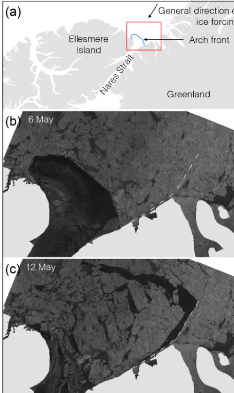
Sentinel-1 SAR backscatter imagery captured the location and breakup of the ice arch in Nares Strait in 2017 (Fig. 10). This breakup event occurred relatively early compared with past events (Kwok, 2005), partly in response to thinner ice conditions and northerly winds (Moore and McNeil, 2018). The arch appeared stable on 6 May (Fig. 10b), before even-tually failing sometime before 12 May (Fig. 10c) as seen in the SAR backscatter images. The interferograms revealed the ice deformation around the location of fracture up until the failure event. As seen in the interferograms, the ice arch fea-tures various levels of centimeter- to meter-scale deformation and fractures prior to breakup, resulting in fringe
Figure 8. (a)Sentinel-1 interferograms derived from image pairs acquired over the Kara Sea between March and May 2017. Numbers on images represent date ranges. The colors blue, green, yellow, and red signify the months of February–May.(b, c, d)Three enlarged areas identified in(a)are further discussed in the text.
whole arch appears to fail through shear motion along this same fault (Fig. 11f).
4 Discussion
4.1 Validating stability zones with areas of known ice stability
The InSAR technique used to map bottomfast sea ice was thoroughly validated in several regions by Dammann et al. (2018c). The high stability of these regions can be inferred from the ice resting on the seafloor. However, other stability zones (i.e., stabilized and nonstabilized ice) are based on rel-ative stability, in terms of whether the ice is anchored or shel-tered. Determining absolute stability (i.e., whether an area is stable enough for a specific use, such as ice roads) would be problematic using fringe density alone. This is because there
are many factors that affect fringe density in addition to sta-bility, including changing wind and ocean currents, satellite viewing geometry, and the prevalent mode of ice deforma-tion (Dammann et al., 2016). A measure of whether ice is practically stable would also depend on specific stakeholders and their dependence on stability. For example, on shorter timescales, industry ice roads would be able to accommo-date less strain than community ice trails, due to differ-ent modes of transportation and user-specific needs. Further steps to identify such thresholds are outlined in Dammann et al. (2018a).
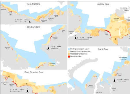
Figure 9.InSAR-derived map of nonstabilized and stabilized landfast ice and bottomfast ice from Sentinel-1 image pairs, acquired predom-inantly between March and May 2017. Letters A–G mark areas discussed in the text. Land is masked out in light grey. This map of stability zones is subject to limitations and uncertainties outlined in the text.
(8, 15, and 17 April) along the Beaufort Sea coast. These images exhibit, in certain locations, a sharp discontinuity in backscatter, which can identify the location of the landfast ice edge (see white arrows in Fig. 12a).
The landfast ice edge identified using backscatter is con-sistent with the three nodes (A–C) identified by Mahoney et al. (2007, 2014; our Fig. 12b). These nodes signify a per-sistent landfast ice edge, believed to be a result of reoc-curring grounded ice features (Mahoney et al., 2014). The ice shoreward of these three nodes is expected to be stabi-lized, because grounded ridges are known to stabilize land-fast ice, leading to reduced strain shoreward of the grounding points (Mahoney et al., 2007; Druckenmiller, 2011). Interfer-ograms exhibit a phase response, suggesting stabilized ice di-rectly shoreward of nodes A and C (Fig. 12c). Here, node A is known to correspond to the location of large grounded ridges, offering stability to the ice cover (Meyer et al., 2011). Nodes B and C are also expected to be regions of persistent grounded ridges since the nodes coincide roughly with the 20 m isobath (Mahoney et al., 2014). However, ice directly shoreward of node B appears nonstabilized, with stabiliza-tion only further in. This may be due to the reduced keel
depth of ridges in 2017 or the possibly reduced grounding strength of ridges present in Node B. Certain sections of the border between stabilized and nonstabilized ice extend rel-atively far from the coast (see black arrows in Fig. 12d). At these points, the stability is higher than adjacent areas with the same distance from shore. This is consistent with increased stability behind grounded ridges.
Although the landfast ice edge can in some instances be mapped using a single backscatter image, stabilized ice can-not easily be discriminated from nonstabilized ice. This is apparent when comparing grounding locations as obtained with InSAR with backscatter images (see black arrows in Fig. 12a). It is also worth noting that relying on backscat-ter to discriminate landfast or drifting ice only works in some cases. There must be noticeable differences in backscatter be-tween landfast and drifting ice, or a severely deformed land-fast ice edge as a result of shear interaction with the pack ice (Druckenmiller et al., 2013).
deter-Figure 10.Map of Nares Strait(a), and Sentinel-1 backscatter im-ages over the 2017 ice arch (blue line ina) before(b)and after(c) failure. The line of failure is identified in(c)and marked as a dashed line in(b, c). Land is masked out in light gray.
mined due to limited data availability in the region, and one interferogram had to be acquired as early as February, be-fore this region had stabilized. Stabilized ice is expected in this region, which features a large shoal, earlier ice formation than surrounding areas, and grounded ridges (Selyuzhenok et al., 2015). The location of this large shoal, along with smaller ones, are obtained from Jakobsson et al. (2012) and displayed in Fig. 13b. Here, it is apparent that even some of the smaller shoals are associated with stabilized ice (see B and C in Fig. 13b). It is also clear that the extensive stabi-lized ice that stretches out halfway between Great Lakhovsky Island and Stolbovoy Island is potentially anchored between the coast and the shallow areas (see D in Fig. 13b).
4.2 Methodological limitations for mapping stability zones
There are a number of sources of uncertainty that affect our map of landfast ice and its relative stability. Dammann et al. (2018c) have determined that, in some instances, bottom-fast ice has to be approximated on the subkilometer scale due to ambiguities associated with low fringe density or fringes parallel to the bottomfast ice edge. We also acknowledge that small islands or sandbars not represented by our landmask may be erroneously identified as bottomfast ice. We have re-duced such errors by not mapping areas that appear to be low-lying land in the SAR backscatter images. However, dis-criminating between ice and low-lying land can be difficult based on strictly SAR. Here, other remote-sensing systems such as optical systems could be applied to further reduce biases from coastline errors. In areas where the landmask does not appear to fit the coastline due to errors or coast-line changes, mapping intricate coastal morphology can be a time-consuming task – hence mapping on a pan-Arctic scale will inevitably contain inaccuracies. It is also worth mention-ing that the other stability zones are mapped against the land-mask, also likely resulting in errors. However, as the extent of these zones are larger, the relative contribution of such errors will be much smaller.
Figure 11.Interferogram over the Nares Strait ice arch in 2017, covering the time period 6–12 April(a). Smaller panels show consecutive interferograms within the box for 12–18 April(b), 18–24 April(c), 24–30 April(d), 30 April–6 May(e), and 6–12 May(f). Dashed line represents the line separating fast and moving ice in Fig. 12c. The black arrows in(d)indicate fringe patterns further discussed in the text. Land is masked out in light gray.
likely require a different set of evaluation criteria for fringes, depending on regions. Additional data such as bathymetry would also likely strengthen this analysis.
We have focused on some examples with possibly subop-timal classification. One potential candidate for reclassifica-tion is landfast ice in sheltered bays, such as the Khatanga Gulf in the western Laptev Sea, which exhibited predomi-nantly high fringe densities (Fig. 7a). Hence, the Khatanga Gulf was largely identified as nonstabilized, despite being nearly landlocked (Fig. 9). Due to the shallow water in this region, it is likely that the high fringe density is caused in part by vertical motion associated with tides and coastal setup. Since vertical motion has less impact on stability in well-confined landfast ice, such examples suggest the poten-tial need for an additional zone of stability, allowing higher fringe densities in coastally confined regions. Such additional classification would depend on other data sets such as a land-mask or bathymetry to identify the level of restricted ice movement in response to likely forcing conditions. Another, larger-scale example is the eastern Laptev sea, which is an area of landfast ice sheltered by the New Siberian Islands and is typically considered stable (Eicken et al., 2005). However, based on relatively high fringe density, particularly offshore
of the Lena Delta, we classified much of the landfast ice in this region as nonstabilized (Fig. 9). This suggests the crite-ria for stabilized ice used in this analysis is different than in Eicken et al. (2005) and can provide new information related to stability in the region. Based on the overall fringe counts and patterns, the majority of the phase response is due to lateral displacement and potentially only partially due to ver-tical displacement (circular fringe patterns with low density – see Dammann et al., 2016) due to tidal motion. It is pos-sible that landfast ice in this region may be less stable than previously thought, and that a partially stabilized zone may be appropriate. This would be consistent with a recent SAR backscatter analysis of landfast ice in the Laptev Sea (Se-lyuzhenok et al., 2017), which showed that areas identified as landfast ice in operational ice charts may actually contain pockets of partly mobile ice. This was shown for the month after initial landfast ice formation, but could possibly result in more dynamic ice throughout spring due to reduced ice thickness.
Figure 12. (a)Sentinel-1 backscatter images over the western Beaufort Sea. White arrows signify the landfast ice edge as identified by contrasting backscatter.(b) Landfast ice edge occurrence mapped for the period 1996–2008 over the Alaska Beaufort Sea (Mahoney et al., 2014). Light red circles correspond to areas of frequent landfast ice edge formation, referred to as “nodes”.(c)Interferograms between mid-April and mid-May 2017.(d)Different stability zones derived from(c). Potential grounding points as identified in(d)are marked with black arrows in(d, a). Land is masked out in light gray.
interaction with pack ice, there may be little difference in fringe spacing between landfast ice seaward and shoreward of stabilizing anchor points. Without evaluating the phase re-sponse for each area of interest in detail during different forc-ing scenarios, it may be difficult to understand under what conditions the ice remains stable. Classification of stability based on relative differences in fringe density is also compli-cated by the use of nonsimultaneous interferograms to pro-vide complete coverage of a region. The interferograms used here were obtained as close to maximum ice extent and
Figure 13. (a)Sentinel-1 interferograms over Laptev Sea near Stolbovoy Island between February and May 2017.(b)Outlined nonstabilized (light orange) and stabilized (dark orange) ice. Shallow areas (<10 m; Jakobsson et al., 2012) are marked with gray cross hatching. Stabilized ice that is likely supported by grounding near shallow features are marked A–D and further discussed in the text. Land is masked out in light gray.
Sentinel-1 IW imagery is predominantly acquired over land, so it is likely not possible to construct interferograms away from the coast, for extensive landfast ice approaching the 250 km IW swath, such as that in the East Siberian Sea. Data availability further restricts the temporal baseline be-tween images to a minimum of 12 days, though this now rep-resents a shorter period than past work identifying landfast ice (Mahoney et al., 2004; Meyer et al., 2011; Dammann et al., 2016). Further studies should investigate the effect of dif-ferent temporal baselines on the stability product. A shorter baseline will result in higher temporal resolution. However, with a shorter baseline (e.g., Sentinel-1 6-day baseline), map-ping of the seaward landfast ice edge may incorporate sta-tionary pack ice. A longer baseline will result in lower inter-ferometric coherence. With a 12-day baseline, some regions, such as the Kotzebue Sound region, already feature consis-tent coherence loss. Such regions can most often be identified through a spatially inconsistent progression, from high to a complete loss of coherence. In such cases, the mapping of landfast ice type boundaries is not possible. It is worth men-tioning that this technique can only be used before the onset of melt, when widespread coherence loss occurs. Therefore, it is not possible to evaluate the retreat of bottomfast ice or the reduction of ice stability in response to melt.
5 Conclusion
In a time of rapidly changing sea ice conditions and contin-ued interest in the Arctic from a range of stakeholders, we stress the need for new assessment strategies to enable safe and efficient use of sea ice. InSAR is gaining growing atten-tion in the sea ice scientific community, and here we demon-strate its value for identifying zones of landfast ice stabil-ity. We are also highlighting the application of InSAR for the development of operational sea ice information products,
for both long-term strategic planning and short-term tactical decisions. Using interferograms generated by a standardized workflow, we show that three stability zones of landfast ice can be identified based on fringe density and continuity, in-dicative of differential ice motion occurring between SAR acquisitions. Along the Beaufort Sea coast of Alaska, we find that the landfast ice regime can be well described with three stability zones: bottomfast ice, where the sea ice is frozen to or resting on the seabed; stabilized ice, which is floating but sheltered by coastlines or anchored by islands or grounded ridges; and nonstabilized ice, which represent floating exten-sions seaward of any anchoring points. These findings are supported by comparison with the location of stable nodes, identified through analysis of hundreds of landfast ice edge positions over the period 1996–2008. Not only does this pro-vide some validation of our results, but it demonstrates the ability of InSAR to capture useful information in just two snapshots, compared to previously requiring analysis over many years.
The use of a standardized workflow facilitates large-scale application of this approach, which we demonstrate on a near-pan-Arctic scale using 52 Sentinel-1 acquisition pairs during spring 2017. This has allowed us to map the same zones of landfast ice in the Beaufort, Chukchi, East Siberian, Laptev, and Kara seas. To our knowledge, our results repre-sent the first mapping of bottomfast ice extent at this scale and the first attempt to map the extents of different landfast ice stability zones on any scale. It also enabled us to estimate and compare the total area covered by each stability zone in each marginal sea. However, we note that these comparisons are based on the assumptions that the landfast ice regimes in all these seas can be well described by the same three sta-bility zones. Although the delineation of different zones can be subjective, in particular in the Russian Arctic, our results clearly show that not all landfast ice is equally stable. Here, InSAR is potentially able to detect small-scale motion up to hundreds of kilometers from the shore that have previously been overlooked. In addition, there are uncertainties associ-ated with the exact mapping of stability zones – in particular in terms of the exact delineation between stabilized and non-stabilized ice in the East Siberian and Laptev seas. Here, the boundaries between stabilized and nonstabilized ice are more difficult to discriminate, likely due to fewer pinning points where the ice is grounded or supported. Therefore, what we present here is not an operational ice chart, but the ability and application to discriminate stability classes on a pan-Arctic scale using InSAR.
The method presented in this work has a broad set of potential applications for monitoring, including subsea per-mafrost, biological habitats both beneath and above the ice surface, and ice use by a range of stakeholders. Bottomfast ice is important because it helps the aggregation of sub-sea permafrost, which serves to constrain the location of permafrost-rich shorelines. Utilizing InSAR, it is likely pos-sible to monitor changes in bottomfast ice over time, with significant implications for erosion and spring flooding and the release of methane hydrates. We argue that the utility of InSAR and its potential applications also extend to maritime activities and shipping. With regards to the latter, vessel traf-fic typically does not traverse landfast ice. However, the as-sessment of landfast ice stability and spatiotemporal extent can potentially aid the management of conflicting ice uses such as in the case of the access route to the Voisey’s Bay Mine in the Canadian Arctic, which cuts through the land-fast ice that is part of a traditional Nunatsiavummiut use area (Bell et al., 2014).
With respect to ice users, sea ice navigation near or through landfast sea ice is presently predominately supported by sea ice charts used to map areas occupied by landfast ice. However, these charts do not provide information about the relative stability of the ice. The information provided here would likely be useful in the context of navigation and sup-port of on-ice operations. The InSAR-based approach
de-scribed here can potentially provide support by identifying the following stability-related features:
1. low-stability ice that may break off and drift into ship-ping lanes,
2. grounded ridges that may be problematic for ice navi-gation, but at the same time may provide added stability for on-ice operations,
3. stable areas to use for equipment staging by coastal community hunters and industry,
4. bottomfast ice for development of ice roads for trans-portation of heavy loads.
We further demonstrate the scientific and operational value of InSAR over sea ice through the examination of interfero-grams of ice arches. In this context, they can be considered part of an additional stability zone of quasi-landfast ice (i.e., temporarily stabilized pack ice). Preliminary analysis of the Nares Strait ice arch in 2017 suggests that interferograms may reveal precursors to the failure of ice arches. We fur-ther speculate that InSAR tools can be developed to inform stakeholders of changing landfast ice stability and ice move-ment. Such applications would have potential value for an early warning system designed to alert ice users of hazards related to ice movement and breakout events. The use of in-verse modeling may further help derive the small-scale strain field from interferograms, which may improve our ability to predict their failure. We expect that InSAR can provide valu-able information for stakeholders, enabling the tracking of ice dynamics and stability on seasonal timescales. The abil-ity to provide stabilabil-ity information to stakeholders also opens up for the development of operational guidelines in terms of what stability zones should be prioritized or avoided.
Data availability. Sentinel-1 data from this analysis can be ob-tained free of charge from the Copernicus Open Access Hub (https://scihub.copernicus.eu/, European Space Agency, 2019) or the Alaska Satellite Facility Vertex interface (https://vertex.daac.asf. alaska.edu/, Alaska Satellite Facility, 2018). See the Supplement for a full list of images used. The shapefiles for bottomfast, stabilized, and nonstabilized ice used for the final map shown in Fig. 9 are included in the Supplement.
Supplement. The supplement related to this article is available online at: https://doi.org/10.5194/tc-13-557-2019-supplement.
Author contributions. DOD conducted the interferometric process-ing and analysis and drafted the initial manuscript. LEBE and ARM provided critical guidance on all aspects of the analysis and manuscript. HE provided expertise relevant to sea ice processes in different Arctic regions. FJM provided expertise relevant to the interferometric processing and analysis. All co-authors also pro-vided valuable recommendations and corrections resulting in the final manuscript.
Competing interests. The authors declare that they have no conflict of interest.
Acknowledgements. This work was funded by the Swedish Na-tional Space Agency (no. 192/15). Sentinel-1 data are provided free of charge by the European Union Copernicus program and were downloaded from the NASA Alaska Satellite Facility (ASF) SAR Distributed Active Archive Center (DAAC). We thank Bill Hauer (ASF) for valuable data support and Christopher Stevens (SRK Consulting) and Joost van der Sanden (Canada Centre for Mapping and Earth Observation) for valuable guidance. We thank Nate Bauer (International Arctic Research Center) and two anonymous re-viewers who substantially contributed to improving this manuscript.
Edited by: Lars Kaleschke
Reviewed by: two anonymous referees
References
ACIA: Impacts of a Warming Arctic, Arctic Climate Impact As-sessment, Cambridge University Press, Cambridge, UK, 144 pp., 2004.
Alaska Satellite Facility: NASA ASF Distributed Active Archive Center (DAAC) Vertex interface, available at: https://vertex.daac. asf.alaska.edu/, last access: 28 May 2018.
Alexandrov, V. Y., Martin, T., Kolatschek, J., Eicken, H., Kreyscher, M., and Makshtas, A. P.: Sea ice circulation in the Laptev Sea and ice export to the Arctic Ocean: Results from satellite remote sensing and numerical modeling, J. Geophys. Res., 105, 17143– 17159, 2000.
Aporta, C. and Higgs, E.: Satellite culture – Global po-sitioning systems, inuit wayfinding, and the need for a
new account of technology, Curr. Anthropol., 46, 729–753, https://doi.org/10.1086/432651, 2005.
Arctic Council: Arctic marine shipping assessment, Protection of the Arctic Marine Environment Working Group (PAME), Akureyri, Island, 190 pp., 2009.
Are, F. and Reimnitz, E.: An overview of the Lena River Delta setting: geology, tectonics, geomorphology, and hydrology, J. Coastal Res., 16, 1083–1093, 2000.
Bailey, W.: Oceanographic features of the Canadian Archipelago, J. Fish. Res. Board Can., 14, 731–769, 1957.
Bamler, R. and Hartl, P.: Synthetic aperture radar interferometry, In-verse Probl., 14, 4, https://doi.org/10.1088/0266-5611/14/4/001, 1998.
Barber, D., Babb, D., Ehn, J., Chan, W., Matthes, L., Dalman, L., Campbell, Y., Harasyn, M., Firoozy, N., and Theriault, N.: In-creasing mobility of high Arctic sea ice increases marine haz-ards off the east coast of Newfoundland, Geophys. Res. Lett., 45, 2370–2379, https://doi.org/10.1002/2017GL076587, 2018. Bell, T., Briggs, R., Bachmayer, R., and Li, S.: Augmenting Inuit
knowledge for safe sea-ice travel – The SmartICE information system, 2014 Oceans’14 St. John’s, Newfoundland, Canada, 14– 19 September 2014, 1–9, 2014.
Berg, A., Dammert, P., and Eriksson, L. E. B.: X-Band Interferometric SAR Observations of Baltic Fast Ice, IEEE T. Geosci. Remote, 53, 1248–1256, https://doi.org/10.1109/TGRS.2014.2336752, 2015.
Comiso, J. C. and Hall, D. K.: Climate trends in the Arctic as observed from space, Wiley Interdisciplinary Reviews: Climate Change, 5, 389-409, https://doi.org/10.1002/wcc.277, 2014. Dammann, D. O.: Arctic sea ice trafficability – new strategies for a
changing icescape, PhD thesis, Department of Geosciences, Uni-versity of Alaska Fairbanks, Fairbanks, Alaska, USA, 217 pp., 2017.
Dammann, D. O., Eicken, H., Meyer, F., and Mahoney, A.: As-sessing small-scale deformation and stability of landfast sea ice on seasonal timescales through L-band SAR interferometry and inverse modeling, Remote Sens. Environ., 187, 492–504, https://doi.org/10.1016/j.rse.2016.10.032, 2016.
Dammann, D. O., Eicken, H., Saiet, E., Mahoney, A., Meyer, F., and George, J. C.: Traversing sea ice – linking sur-face roughness and ice trafficability through SAR polarime-try and interferomepolarime-try IEEE J. Sel. Top Appl., 11, 416–433, https://doi.org/10.1109/JSTARS.2017.2764961, 2017.
Dammann, D. O., Eicken, H., Mahoney, A., Meyer, F., and Betcher, S.: Assessing sea ice trafficability in a changing Arctic, Arctic, 71, 59–75, https://doi.org/10.14430/arctic4701, 2018a.
Dammann, D. O., Eicken, H., Mahoney, A., Meyer, F., Frey-mueller, J., and Kaufman, A. M.: Evaluating landfast sea ice stress and fracture in support of operations on sea ice us-ing SAR interferometry, Cold Reg. Sci. Technol., 149, 51–64, https://doi.org/10.1016/j.coldregions.2018.02.001, 2018b. Dammann, D. O., Eriksson, L. E. B., Mahoney, A., Stevens, C. W.,
Van der Sanden, J., Eicken, H., Meyer, F., and Tweedie, C.: Map-ping Arctic bottomfast sea ice using SAR interferometry, Remote Sens., 10, 720, https://doi.org/10.3390/rs10050720, 2018c. Dammert, P. B. G., Lepparanta, M., and Askne, J.: SAR
Dierking, W., Lang, O., and Busche, T.: Sea ice local sur-face topography from single-pass satellite InSAR measure-ments: a feasibility study, The Cryosphere, 11, 1967–1985, https://doi.org/10.5194/tc-11-1967-2017, 2017.
Druckenmiller, M. L.: Alaska shorefast ice: interfacing geophysics with local sea ice knowledge and use, PhD thesis, University of Alaska Fairbanks, Fairbanks, Alaska, 210 pp., 2011.
Druckenmiller, M. L., Eicken, H., George, J. C., and Brower, L.: Trails to the whale: reflections of change and choice on an Iñu-piat icescape at Barrow, Alaska, Polar Geography, 36, 5–29, https://doi.org/10.1080/1088937X.2012.724459, 2013.
Eguíluz, V. M., Fernández-Gracia, J., Irigoien, X., and Duarte, C. M.: A quantitative assessment of Arctic shipping in 2010–2014, Scientific Reports, 6, 30682, https://doi.org/10.1038/srep30682, 2016.
Eicken, H. and Mahoney, A. R.: Sea Ice: Hazards, Risks, and Impli-cations for Disasters, in: Coastal and Marine Hazards, Risks, and Disasters, edited by: Ellis, J. T., Sherman, D. J., and Shroder, J. F., Elsevier Inc., Amsterdam, Netherlands, 381–399, 2015. Eicken, H., Dmitrenko, I., Tyshko, K., Darovskikh, A.,
Dierk-ing, W., Blahak, U., Groves, J., and Kassens, H.: Zona-tion of the Laptev Sea landfast ice cover and its impor-tance in a frozen estuary, Global Planet. Change, 48, 55–83, https://doi.org/10.1016/j.gloplacha.2004.12.005, 2005.
Eicken, H., Lovecraft, A. L., and Druckenmiller, M. L.: Sea-Ice Sys-tem Services: A Framework to Help Identify and Meet Informa-tion Needs Relevant for Arctic Observing Networks, Arctic, 62, 119–136, https://doi.org/10.14430/arctic126, 2009.
Eicken, H., Jones, J., Meyer, F., Mahoney, A., Druckenmiller, M. L., Rohith, M., and Kambhamettu, C.: Environmental security in Arctic ice-covered seas: from strategy to tactics of hazard identi-fication and emergency response, Mar. Technol. Soc. J., 45, 37– 48, https://doi.org/10.4031/MTSJ.45.3.1, 2011.
European Space Agency: Copernicus Programme, Open Access Hub, available at: https://scihub.copernicus.eu/, last access: 4 February 2019.
Ferretti, A., Monti-Guarnieri, A., Prati, C., Rocca, F., and Massonet, D.: InSAR Principles-Guidelines for SAR Interferometry Pro-cessing and Interpretation, ESA Publications, TM-19, 2007. Fienup-Riordan, A. and Rearden, A.: The ice is always changing:
Yup’ik understandings of sea ice, past and present, in: SIKU: knowing Our Ice: Documenting Inuit Sea Ice knowledge and Use, edited by: Krupnik, I., Aporta, C., Gearheard, S., Laidler, G., and Holm, L. K., Springer, New York, 295–320, 2010. Ford, J. D., Pearce, T., Gilligan, J., Smit, B., and Oakes, J.:
Climate change and hazards associated with ice use in northern Canada, Arct. Antarct. Alp. Res., 40, 647–659, https://doi.org/10.1657/1523-0430(07-040)[FORD]2.0.CO;2, 2008.
Giles, A. B., Massom, R. A., and Lytle, V. I.: Fast-ice dis-tribution in East Antarctica during 1997 and 1999 deter-mined using RADARSAT data, J. Geophys. Res., 113, C02S14, https://doi.org/10.1029/2007JC004139, 2008.
Goldstein, R. M. and Werner, C. L.: Radar interferogram filter-ing for geophysical applications, Geophys. Res. Lett., 25, 4035– 4038, https://doi.org/10.1029/1998GL900033, 1998.
Haas, C. and Howell, S. E.: Ice thickness in the North-west Passage, Geophys. Res. Lett., 42, 7673–7680, https://doi.org/10.1002/2015GL065704, 2015.
Hibler, W., Hutchings, J., and Ip, C.: Sea-ice arching and multi-ple flow states of Arctic pack ice, Ann. Glaciol., 44, 339–344, https://doi.org/10.3189/172756406781811448, 2006.
Hirose, T., Kapfer, M., Bennett, J., Cott, P., Manson, G., and Solomon, S.: Bottomfast Ice Mapping and the Measurement of Ice Thickness on Tundra Lakes Using C-Band Synthetic Aper-ture Radar Remote Sensing, JAWRA J. Am. Water Resour. As., 44, 285–292, https://doi.org/10.1111/j.1752-1688.2007.00161.x, 2008.
Howell, S. E., Wohlleben, T., Dabboor, M., Derksen, C., Ko-marov, A., and Pizzolato, L.: Recent changes in the exchange of sea ice between the Arctic Ocean and the Canadian Arc-tic Archipelago, J. Geophys. Res.-Oceans, 118, 3595–3607, https://doi.org/10.1002/jgrc.20265, 2013.
Hui, F., Zhao, T., Li, X., Shokr, M., Heil, P., Zhao, J., Zhang, L., and Cheng, X.: Satellite-Based Sea Ice Naviga-tion for Prydz Bay, East Antarctica, Remote Sens., 9, 518, https://doi.org/10.3390/rs9060518, 2017.
Jakobsson, M., Mayer, L., Coakley, B., Dowdeswell, J. A., Forbes, S., Fridman, B., Hodnesdal, H., Noormets, R., Pedersen, R., and Rebesco, M.: The international bathymetric chart of the Arctic Ocean (IBCAO) version 3.0, Geophys. Res. Lett., 39, L12609, https://doi.org/10.1029/2012GL052219, 2012.
Johannessen, O. M., Alexandrov, V., Frolov, I. Y., Sandven, S., Pettersson, L. H., Bobylev, L. P., Kloster, K., Smirnov, V. G., Mironov, Y. U., and Babich, N. G.: Remote sensing of sea ice in the Northern Sea Route: studies and applications, Springer Sci-ence & Business Media, Chichester, United Kingdom, 2006. Jones, J. M., Eicken, H., Mahoney, A. R., Rohith, M. V.,
Kamb-hamettu, C., Fukamachi, Y., Ohshima, K. I., and George, J. C.: Landfast sea ice breakouts: Stabilizing ice features, oceanic and atmospheric forcing at Barrow, Alaska, Cont. Shelf Res., 126, 50–63, https://doi.org/10.1016/j.csr.2016.07.015, 2016. Krupnik, I., Aporta, C., Gearheard, S., Laidler, G. J., and Holm, L.
K.: SIKU: knowing our ice, Springer, New York, 2010. Kwok, R.: Variability of Nares Strait ice flux, Geophys. Res. Lett.,
32, L24502, https://doi.org/10.1029/2005GL024768, 2005. Kwok, R.: Exchange of sea ice between the Arctic Ocean and the
Canadian Arctic Archipelago, Geophys. Res. Lett., 33, L16501, https://doi.org/10.1029/2006GL027094, 2006.
Kwok, R., Toudal Pedersen, L., Gudmandsen, P., and Pang, S.: Large sea ice outflow into the Nares Strait in 2007, Geophys. Res. Lett., 37, L03502, https://doi.org/10.1029/2009GL041872, 2010.
Li, S., Shapiro, L., McNutt, L., and Feffers, A.: Application of Satel-lite Radar Interferometry to the Detection of Sea Ice Deforma-tion, Journal of the Remote Sensing Society of Japan, 16, 67–77, https://doi.org/10.11440/rssj1981.16.153, 1996.
Lovecraft, A. L. and Eicken, H.: North by 2020: perspectives on Alaska’s changing social-ecological systems, University of Alaska Press, Fairbanks, Alaska, 2011.
Mahoney, A., Eicken, H., Graves, A., Shapiro, L., and Cotter, P.: Landfast sea ice extent and variability in the Alaskan Arctic de-rived from SAR imagery, in: Proceedings of the International Geoscience and Remote Sensing Symposium IGARSS, Anchor-age, AK, USA, 20–24 September 2004, 2146–2149, 2004. Mahoney, A., Eicken, H., and Shapiro, L.: How fast is landfast
ice at Barrow, Alaska, Cold Reg. Sci. Technol., 47, 233–255, https://doi.org/10.1016/J.Coldregions.2006.09.005, 2007. Mahoney, A., Eicken, H., Gaylord, A. G., and Gens, R.: Landfast
sea ice extent in the Chukchi and Beaufort Seas: The annual cy-cle and decadal variability, Cold Reg. Sci. Technol., 103, 41–56, https://doi.org/10.1016/J.Coldregions.2014.03.003, 2014. Marbouti, M., Praks, J., Antropov, O., Rinne, E., and
Lep-päranta, M.: A Study of Landfast Ice with Sentinel-1 Repeat-Pass Interferometry over the Baltic Sea, Remote Sens., 9, 833, https://doi.org/10.3390/rs9080833, 2017.
Meier, W. N., Hovelsrud, G. K., Oort, B. E., Key, J. R., Ko-vacs, K. M., Michel, C., Haas, C., Granskog, M. A., Ger-land, S., and Perovich, D. K.: Arctic sea ice in transfor-mation: A review of recent observed changes and impacts on biology and human activity, Rev. Geophys., 52, 185–217, https://doi.org/10.1002/2013RG000431, 2014.
Melling, H.: Sea ice of the northern Canadian Arc-tic Archipelago, J. Geophys. Res., 107, 3181, https://doi.org/10.1029/2001JC001102 2002.
Meyer, F. J., Mahoney, A. R., Eicken, H., Denny, C. L., Druckenmiller, H. C., and Hendricks, S.: Mapping arctic landfast ice extent using L-band synthetic aperture radar interferometry, Remote Sens. Environ., 115, 3029–3043, https://doi.org/10.1016/J.Rse.2011.06.006, 2011.
Meyer, F. J., McAlpin, D., Gong, W., Ajadi, O., Arko, S., Webley, P., and Dehn, J.: Integrating SAR and de-rived products into operational volcano monitoring and deci-sion support systems, ISPRS J. Photogramm., 100, 106–117, https://doi.org/10.1016/j.isprsjprs.2014.05.009, 2015.
Moore, G. and McNeil, K.: The early collapse of the 2017 Lincoln Sea ice arch inresponse to anomalous sea ice and wind forcing, Geophys. Res. Lett., 45, 8343–8351, https://doi.org/10.1029/2018GL078428, 2018.
Morris, K., Li, S., and Jeffries, M.: Meso-and microscale sea-ice motion in the East Siberian Sea as deter-mined from ERS-I SAR data, J. Glaciol., 45, 370–383, https://doi.org/10.3189/S0022143000001878, 1999.
Muckenhuber, S. and Sandven, S.: Open-source sea ice drift algo-rithm for Sentinel-1 SAR imagery using a combination of feature tracking and pattern matching, The Cryosphere, 11, 1835–1850, https://doi.org/10.5194/tc-11-1835-2017, 2017.
Onstott, R. G.: SAR and scatterometer signatures of sea ice, in: Mi-crowave remote sensing of sea ice, 68, 73–104, 1992.
Orviku, K., Jaagus, J., and Tõnisson, H.: Sea ice shaping the shores, J. Coastal Res., SI64, 681–685, 2011.
Potter, R., Walden, J., and Haspel, R.: Design and construction of sea ice roads in the Alaskan Beaufort Sea, Offshore Technology Conference, Houston, Texas, 1981.
Reimnitz, E., Dethleff, D., and Nürnberg, D.: Contrasts in Arctic shelf sea-ice regimes and some implications: Beau-fort Sea versus Laptev Sea, Mar. Geol., 119, 215–225, https://doi.org/10.1016/0025-3227(94)90182-1, 1994.
Screen, J. A. and Simmonds, I.: The central role of diminishing sea ice in recent Arctic temperature amplification, Nature, 464, 1334–1337, https://doi.org/10.1038/nature09051, 2010. Selyuzhenok, V., Krumpen, T., Mahoney, A., Janout, M.,
and Gerdes, R.: Seasonal and interannual variability of fast ice extent in the southeastern Laptev Sea between
1999 and 2013, J. Geophys. Res.-Oceans, 120, 7791–7806, https://doi.org/10.1002/2015JC011135, 2015.
Selyuzhenok, V., Mahoney, A., Krumpen, T., Castellani, G., and Gerdes, R.: Mechanisms of fast-ice development in the south-eastern Laptev Sea: a case study for win-ter of 2007/08 and 2009/10, Polar Res., 36, 1411140, https://doi.org/10.1080/17518369.2017.1411140, 2017. Smith, T. G.: Polar bear predation of ringed and bearded seals
in the land-fast sea ice habitat, Can. J. Zool., 58, 2201–2209, https://doi.org/10.1139/z80-302, 1980.
Solomon, S. M., Taylor, A. E., and Stevens, C. W.: Nearshore ground temperatures, seasonal ice bonding, and permafrost for-mation within the bottom-fast ice zone, Mackenzie Delta, NWT, in: Proceedings of the Ninth International Conference on Per-mafrost, University of Alaska Fairbanks, Fairbanks, Alaska, USA, 29 June–3 July 2008, 1675–1680, 2008.
Stephenson, S. R., Smith, L. C., and Agnew, J. A.: Divergent long-term trajectories of human access to the Arctic, Nat. Clim Change, 1, 156–160, https://doi.org/10.1038/Nclimate1120, 2011.
Stevens, C. W.: Controls on Seasonal Ground Freezing and Per-mafrost in the Near-shore Zone of the Mackenzie Delta, PhD Thesis, NWT, Canada, University of Calgary, 2011.
Stevens, C. W., Moorman, B. J., and Solomon, S. M.: Detection of frozen and unfrozen interfaces with ground penetrating radar in the nearshore zone of the Mackenzie Delta, Canada, in: Proceed-ings of the Ninth International Conference on Permafrost, Uni-versity of Alaska Fairbanks, Fairbanks, Alaska, USA, 29 June– 3 July 2008, 1711–1716, 2008.
Stevens, C. W., Moorman, B. J., and Solomon, S. M.: Interan-nual changes in seasonal ground freezing and near-surface heat flow beneath bottom-fast ice in the near-shore zone, Macken-zie Delta, NWT, Canada, Permafrost Periglac., 21, 256–270, https://doi.org/10.1002/ppp.682, 2010.
Stroeve, J. C., Serreze, M. C., Holland, M. M., Kay, J. E., Malanik, J., and Barrett, A. P.: The Arctic’s rapidly shrinking sea ice cover: a research synthesis, Climatic Change, 110, 1005–1027, https://doi.org/10.1007/S10584-011-0101-1, 2012.
Thomas, D. N.: Sea ice, John Wiley & Sons, Chichester, United Kingdom, 2017.
Tibbles, M., Falke, J. A., Mahoney, A. R., Robards, M. D., and Seitz, A. C.: An In SAR habitat suitability model to identify overwinter conditions for coregonine whitefishes in Arctic lagoons, T. Am. Fish. Soc., 147, 1167–1178, https://doi.org/10.1002/tafs.10111, 2018.
Vincent, F., Raucoules, D., Degroeve, T., Edwards, G., and Abolfazl Mostafavi, M.: Detection of river/sea ice deformation using satel-lite interferometry: limits and potential, Int. J. Remote Sens., 25, 3555–3571, https://doi.org/10.1080/01431160410001688303, 2004.
Werner, C., Wegmüller, U., Strozzi, T., and Wiesmann, A.: Gamma SAR and interferometric processing software, in: Proceedings of the ERS-ENVISAT Symposium, Gothenburg, Sweden, 16– 20 October 2000.
Wilson, K. J., Falkingham, J., Melling, H., and De Abreu, R.: Shipping in the Canadian Arctic: other possible climate change scenarios, Proceedings of the International Geoscience and Re-mote Sensing Symposium IGARSS, Anchorage, AK, USA, 20– 24 September 2004, 1853–1856, 2004.