1DLR – German Aerospace Center, Remote Sensing Technology Institute, Oberpfaffenhofen, 82234 Weßling, Germany 2TUM – Technical University of Munich, 80333 M¨unchen, Germany
Received: 6 May 2011 – Published in Atmos. Meas. Tech. Discuss.: 10 June 2011 Revised: 7 October 2011 – Accepted: 20 November 2011 – Published: 8 December 2011
Abstract. Nadir observations with the shortwave infrared channels of SCIAMACHY on-board the ENVISAT satellite can be used to derive information on atmospheric gases such as CO, CH4, N2O, CO2, and H2O. For the operational level
1b-2 processing of SCIAMACHY data, a new retrieval code BIRRA (Beer InfraRed Retrieval Algorithm) has been de-veloped. BIRRA performs a nonlinear or separable least squares fit (with bound constraints optional) of the measured radiance, where molecular concentration vertical profiles are scaled to fit the observed data. Here we present the forward modeling (radiative transfer) and inversion (least squares op-timization) fundamentals of the code along with the further processing steps required to generate higher level products such as global distributions and time series. Moreover, vari-ous aspects of level 1 (observed spectra) and auxiliary input data relevant for successful retrievals are discussed. BIRRA is currently used for operational analysis of carbon mono-xide vertical column densities from SCIAMACHY channel 8 observations, and is being prepared for methane retrievals using channel 6 spectra. A set of representative CO retrievals and first CH4results are presented to demonstrate BIRRA’s
capabilities.
1 Introduction
Nadir sounding of molecular column densities is well es-tablished in atmospheric remote sensing. For UV instru-ments observing the back-scattered sunlight, the analy-sis is traditionally based on a DOAS (Differential Optical
Correspondence to: S. Gimeno Garc´ıa ([email protected])
Absorption Spectroscopy) methodology that considers the logarithm of the measured signal – essentially the optical depth. This approach has also been successfully applied to SCIAMACHY’s (Scanning Imaging Absorption Spectrom-eter for Atmospheric CHartographY) (Bovensmann et al., 1999; Gottwald and Bovensmann, 2011) near infrared (NIR) channels (Buchwitz et al., 2007; Frankenberg et al., 2005b). Alternatively, the measured radiance spectra can be directly analyzed. This method is common practice in thermal in-frared atmospheric spectroscopy and constitutes the core of the Iterative Maximum Likelihood Method (IMLM) devel-oped by SRON for analysis of SCIAMACHY’s near infrared channels (Gloudemans et al., 2005). Recently, Reuter et al. (2010) also presented an optimum estimation analysis of sun normalized radiances for improved SCIAMACHY CO2
re-trievals and Lerot et al. (2010) applied a direct fitting to nadir viewing UV spectra.
The aim of SCIAMACHY nadir NIR observations is to retrieve information on atmospheric gases such as CO, CH4,
CO2, N2O, or H2O. Ideally, profiles of volume mixing
ra-tioqX(z)or number densitynX(z)=qX(z)·nair(z)of a given
molecule X can be retrieved, wherezrepresents altitude and
nair air number density. However, vertical sounding
inver-sions are generally ill-posed problems, so for weakly ab-sorbing gases it is customary to retrieve only vertical column densities (VCD),
NX≡
Z zTOA
zsrf
nX(z)dz , (1)
wherezsrfis the surface altitude andzTOAthe altitude of top
of the atmosphere (TOA).
In order to have a flexible and robust inversion algorithm for the efficient processing of level-1b to level-2 data, the “Beer InfraRed Retrieval Algorithm” (BIRRA) has been de-veloped at DLR. BIRRA performs a nonlinear least squares
fit of the observed near infrared (sun-normalized) radi-ances. First results including a careful intercomparison with the WFM-DOAS algorithm (Weighting Function Modified DOAS, University of Bremen, Buchwitz et al., 2007) for or-bit 8663 (27 October 2003) have been presented in Schreier et al. (2007). Recently, the BIRRA prototype has been suc-cessfully implemented in version 5 of the level 1b to 2 SCIA-MACHY processor for operational data retrievals.
In this paper, the algorithmic basis of BIRRA and its ap-plication to carbon gas VCD retrievals are presented. The next section reviews the forward model and the inversion ap-proach used in BIRRA as well as further processing steps. Aspects of input data (nb. level 1 issues) and retrieval set-tings are discussed in Sect. 3. Section 4 contains a survey of VCD retrieval results. Conclusions and an outlook are given in Sect. 5. The results presented here have been obtained with the scientific prototype version of BIRRA and may dif-fer from the SCIAMACHY operational product. The em-phasis of this paper is on methodology, where carbon mono-xide and methane retrievals are presented for illustrations. For a discussion of spatial and temporal patterns we refer to, e.g. Buchwitz et al., 2007; Clerbaux et al., 2008; Gloudemans et al., 2006, 2009; de Laat et al., 2006, 2007; Worden et al., 2010; Yurganov et al., 2008. A comprehensive discussion of results for CO and CH4, including validation, will be the
subject of a forthcoming paper.
2 Theory and algorithm
2.1 The forward model – near infrared radiative transfer
For an arbitrary slant path, the intensity (radiance) I at wavenumber ν received by an instrument at s=0 is de-scribed by the equation of radiative transfer (Liou, 1980; Zdunkowski et al., 2007)
I (ν)= Ib(ν)T(ν)−
Z ∞
0
ds0J (ν,s0)∂T(ν;s 0)
∂s0 , (2)
whereIbis an external contribution,T represents the
trans-mission through the atmosphere, andJis the source function comprised of thermal emission and scattering. In the near in-frared, thermal emission of the atmosphere and Earth’s sur-face is negligible compared to the reflected and scattered sun-light. The contribution of molecular (Rayleigh) scattering is far below 1 % and will be neglected. Aerosol and cloud scat-tering may have a significant contribution to the intensity but their effects on the retrieval can be mitigated by proxy mod-eling (see Subsect. 2.3.1, a detailed justification can be found in Frankenberg et al., 2006; Gloudemans et al., 2008). Thus, neglecting scattering, Eq. (2) reduces to Beer’s law for a dou-ble path through the atmosphere
I (ν)= r(ν)
π µIsun(ν)T↑(ν)T↓(ν)
= r(ν)
π µIsun(ν)
exp − sun Z earth
ds0X
m
nm(s0)km ν,p(s0),T (s0) · exp − sat Z earth
ds00X
m
nm(s00)km ν,p(s00),T (s00)
, (3) whereris the surface albedo andT↑andT↓(withT =T↑T↓)
denote transmission between reflection point (e.g. Earth sur-face at altitudezsrf) and observer and between Sun and
re-flection point, respectively.
Assuming spherical symmetry, the path variable s is uniquely related to the altitudez(in a plane–parallel approx-imations0=z0/µwithµ≡cosθfor an observer zenith angle
θ, similarlys00=z00/µ for a solar zenith angle (SZA)θ). kmandnmare the (pressurepand temperatureT dependent) absorption cross section and number density of moleculem. In infrared line-by-line models, the absorption cross section
kmof moleculemis obtained by summing up the contribu-tions from many lines,
km(ν,p,T ) = X
l
Sl(m)(T ) g(ν; ˆνl(m),γl(m)(p,T )), (4) where each individual linel is described by the product of the temperature-dependent line strengthSl(m) and a normal-ized line shape functiongdescribing the broadening mecha-nism. νˆ andγ are line position and half width at half max-imum (HWHM), respectively. The combined effect of pres-sure broadening (corresponding to a Lorentzian line shape) and Doppler broadening (Gaussian line shape) is represented by a Voigt line profile (Schreier, 2011). Line mixing (LM) is not yet considered in BIRRA. Tran et al. (2010) discussed consequences of line mixing in the 2ν3band of methane for
molecular spectroscopy and atmospheric retrievals, conclud-ing that “from the point of view of atmospheric retrievals, neglecting LM with suitable effective line parameters is con-venient and accurate (within current retrieval uncertainties).” The measured spectrum is modeled by convolution of the monochromatic intensity spectrum (3) with a normalized in-strument spectral response functionS
b
I (ν) ≡ (I⊗S)(ν)=
Z ∞
−∞
I ν0×S ν−ν0dν0,
For SCIAMACHY measurements, a Gaussian function is commonly used,
SG(ν,γ ) =
1
γ
ln2
π
1/2
·exp " −ln2 ν γ 2# , (5)
CKD continuum of water (Clough et al., 1989). Jacobians, i.e. derivatives of transmission or radiance spectra with re-spect to the parameters to be retrieved, are obtained by means of automatic differentiation (Griewank, 2000; Hasco¨et and Pascual, 2004). For nadir modeling, refraction is only taken into account for the Sun – Earth path element whereas for the “down-looking” path segment (satellite – Earth’s surface) with viewing angles≤30◦refraction is neglected.
2.2 The inverse problem – least squares
Denoting byαm the molecular scale factor to be estimated and bynpriorm (z)the a-priori (e.g. climatological) number den-sity of moleculem, the total path transmission in Eq. (3) can be written as
T ≡T↑T↓=exp
"
−X
m
τm #
=exp "
−X
m
αmτmprior #
, (6) whereτmis the “true” total optical depth of moleculem(note that for simplicity this equation is written for a non-refractive plane-parallel geometry),
τm(ν) = zTOA Z
zsrf
dz0
1
µ +
1
|µ|
nm(z0)km(ν,z0), (7)
andτmpriorthe a-priori total optical depth computed withnprior (Note that for simplicity this equation is written for a plane-parallel non-refractive atmosphere). From Eq. (6), we have thatτm(ν)=αmτmprior.
If the observation geometry (i.e.zsrf,zTOA,µandµ) is
known, changes in the a-priori molecular cross sectionskm are neglected and it is assumed that the scale factors do not depend on altitude, then, recalling Eq. (1), the “true” VCD of the moleculemcan be written as
Nm = αmNmprior, (8)
whereNmprior=RzzsrfTOAnpriorm (z)dzis the a-priori VCD of the moleculem.
In addition to the scaling factorsαm, the surface albedo
r (generally modeled by a polynomial in wavenumber) is
given by the radiative transfer and instrument model, F(x)≡bI (ν) =
r(ν)
π µIsun(ν) ×exp
"
−X
m
αmτm(ν) #
⊗S(ν,γ )+b(ν) , (10) where the state vectorx≡(α,γ ,r,b)is comprised of molec-ular scale parametersα, and optionally “auxiliary” parame-tersγ ,r,b(the arraysr andbdenote the coefficients of the polynomials in wavenumber).
For the solution of the nonlinear least squares problem, Eq. (9), BIRRA uses solvers provided in the PORT Op-timization Library (Dennis, Jr. et al., 1981, available at http://www.netlib.org/port/) based on a scaled trust region strategy. Furthermore, BIRRA provides the option to use a nonlinear least squares with simple bounds to avoid unphys-ical results, e.g. non-negativity,
min x>0
ky−F(x)k2. (11)
2.2.2 Separable least squares
Note that the surface albedorand the baseline correction(s)
benter the forward modelF, Eq. (10), linearly and the least squares problems, Eqs. (9) and (11), can be reduced to a sep-arable nonlinear least squares problem (Golub and Pereyra, 2003). Splitting the vectorxof parameters to be fitted into a vectorηof nonlinear parameters and a vectorβ of linear parameters, i.e.
x−→(η,β),withx∈Rn,
η≡(α,γ )∈Rp,β≡(r,b)∈Rqandn=p+q, (12) the forward model can be written as
F(x)=
q X
l=1
βlfl(η) , (13)
wherefl:Rp→Rmforl=1,...,q. Combining these
func-tions in a matrix
A(η)≡f1(η),f2(η),...,fq(η)
,withA∈Rm×q, (14)
Equation (9) can be rewritten as a linear least squares prob-lem
min β
ky−Aβk2 (15)
for the vectorβ, that is formally solved by β = ATA
−1
ATy. (16)
Inserting this solution in Eq. (13), the original least squares problem Eq. (9) becomes
min η
y−X
l
ATA−1ATy lfl(η)
2
. (17)
This is a nonlinear least squares problem forηindependent ofβand can be solved in the usual way by means of Gauss– Newton or Levenberg–Marquardt algorithms. Once the op-timumηis found, the linear parameter vectorβis obtained from Eq. (16). The main advantages of this approach are: (i) the nonlinear least squares solver has to iterate only over a reduced fit vectorη; (ii) no initial guess is required for the linear parametersβ; (iii) the size of the Jacobian matrix is reduced.
2.2.3 Jacobians and altitude sensitivity
The Jacobian, J≡∂F/∂x, the partial derivatives of the model function with respect to the fit parameters, is an essential quantity required for Gauss–Newton type itera-tive solvers of nonlinear least squares problems. Although BIRRA performs a least squares fit of vertical column den-sities, derivatives with respect to the (discretized) molecular abundance profiles deliver insight into the sensitivity of the retrievals to different altitude regions in addition to useful hints to the appropriate spectral region selection.
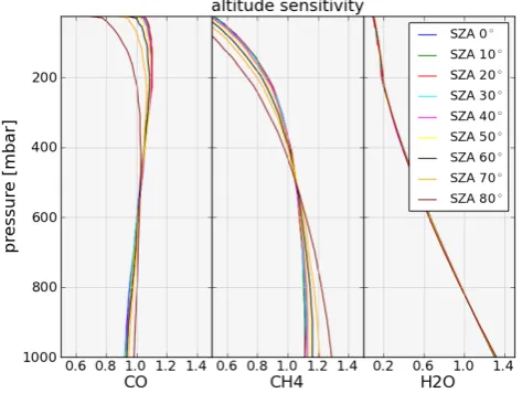
According to Fig. 1, in SCIAMACHY channel 8 both branches of the first CO overtone band at 2.4µm have about the same impact, however, water interference is less signifi-cant in the R-branch between 4250 and 4300 cm−1. Further-more, the plot indicates that the highest altitude sensitivity is located in the troposphere.
For an assessment of altitude sensitivity in the context of profile retrievals, specification of averaging kernels relat-ing the true and estimated state vector (comprisrelat-ing the dis-cretized profile) is customary. In case of column density re-trievals as performed by BIRRA, the state vector is composed of the profile scaling factorsαmof all relevant molecules (and some additional auxiliary parameters). In order to estimate the altitude sensitivity, an approach suggested by Buchwitz et al. (2004) has been used, i.e. a series of BIRRA fits has been performed using synthetic spectra generated with per-turbed CO profiles. DenotingNr(z)the VCD retrieved from the spectrum generated with a profile perturbed at an altitude
Fig. 1. Jacobians[erg/s/(cm2sr cm−1)/ppm]for molecular con-centration profile retrieval in channel 8: CO (top), CH4(mid), and
H2O (bottom). Note the scaling by 106of the CO and CH4
Jaco-bians. The derivatives were calculated using GARLIC for a US standard atmosphere up to 50 km, a Gaussian slit function with
Fig. 2.Altitude sensitivity ofCO(left),CH4(mid), andH2Oin channel 8.
12
Fig. 2. Altitude sensitivity of CO (left), CH4 (mid), and H2O in
channel 8.
z, andNp(z)VCD corresponding to this perturbed profile, the altitude sensitivity is estimated by
A(z) = N
r(z)−N
Np(z)−N , (18)
whereN is the true VCD as in Eq. (1) (the subscript X is omitted for brevity). Fig. 2 confirms the high sensitivity of NIR retrievals in the lower troposphere; furthermore, as pointed out by Buchwitz et al. (2004) and Gloudemans et al. (2008), this sensitivity is depending on the solar zenith angle and, to lesser extent, on the observation angle.
2.3 Postprocessing
In the previous subsections, the basics of forward modeling (radiative transfer) and inversion (least squares optimization) as applied to a single observation have been presented. Here, we discuss further steps necessary to proceed from the fit-ted parameters during the inversion process to “higher level products” such as local and global spatial distributions and temporal evolutions.
2.3.1 Product definition
Since scattering is neglected in the BIRRA forward model, the photon path is considered to be the optical path that so-lar light travels from the top of the atmosphere to the Earth’s surface, and reflected from the surface up to the observer. However, the measured radiance has a high probability of having also a (small or large, depending on the individual conditions) fraction coming from scattering events in the at-mosphere, and consequently, having a photon path different from the pure geometrical one. In addition, the atmospheric conditions are set a-priori to climatological datasets but the actual meteorological conditions (e.g. pressure, temperature)
4
across the CO spectral fitting window, so the amount of CH4
can be determined with high accuracy. Furthermore, CH4is
a well-mixed gas with long life time in the atmosphere and, consequently, it has quite homogeneous global distributions. The deviations of CH4concentrations from the a-priori due
to sources and sinks are rarely bigger than 10 %, far smaller than the deviations of CO that can easily depart by hundreds percent from the reference value over emitting areas. Thus, in terms of CO variability, CH4can be considered as constant
and variations in the retrieved CH4from the expected a-priori
value can be interpreted as the effect of the unconsidered pro-cesses. So, the proxy-normalized CO vertical column density is defined as
xCO≡NCOprior× αCO αCH4
, (19)
whereNCOrepresents the a-priori CO vertical column
den-sity, andαCOandαCH4 are the fitted scaling factors of CO
and CH4, respectively (see Eq. 8). Note that both scaling
factors are retrieved from channel 8 data.
Considering that the retrieval of CH4under the
considera-tions of homogeneity exposed above is equivalent to the re-trieval of the dry air mass, the ratioed quantity xCO is called dry-air column density (Wallace and Livingston, 1990; Yang et al., 2002). For channel 8 retrievals, however, the ice layer that grows over the detector has a different impact on CH4
than on CO retrievals. Thus, the CH4-proxy does not
en-tirely account for the effect of the ice layer and special care has to be taken when correcting for this.
Analogously, using SCIAMACHY channel 6, one can de-fine the dry-air column mixing ratio of CH4as
xCH4≡qCH4prior×αCH4 αCO2
, (20)
whereqCH4prioris the a-priori column mixing ratio of CH4, and αCH4 andαCO2 are the scaling factors of CH4and CO2,
re-spectively. For the target species CH4, the chosen dry-air
proxy is CO2(Frankenberg et al., 2006). All conditions
men-tioned above for the CH4-proxy also hold for the proxy CO2.
Further, CO2 is far more homogeneous (vertical and
hori-zontally) than CH4, and the absorption signatures of target
and proxy species are of comparable magnitude in channel 6, which is desirable but not the case for the CO target with a CH4proxy.
2.3.2 Quality criteria
In order to use the fitted data, a variety of quality crite-ria have to be fulfilled. Convergence of the least squares fit is requested and only moderate solar zenith angles (typ-ically<80dg) are selected. Retrievals with high fit errors are rejected (typicallyε(αCO) <0.5,ε(αCH4) <0.01).
Fur-thermore, for the acceptance or rejection of retrieved data a quantile analysis is performed, i.e. outliers far off the me-dian are rejected. As suggested by Gloudemans et al. (2009), different cloud filters are used over land and over sea: in con-trast to land observations, the NIR albedo of oceans is very low and, as a consequence, the signal-to-noise ratio of cloud free observations is very low. Thus, over oceans the pres-ence of clouds with high albedo significantly enlarges the signal and enables reliable retrievals. Accordingly, only pix-els with cloud fraction higher than 20 % are accepted. Over land, however, the presence of clouds is a source of uncer-tainties, since the radiative transfer model only accounts for one photon path and, in case of partial cloud cover, the ob-served radiances have contributions coming from reflections at the Earth’s surface and from scattering at the cloud layer. Therefore, only observations with cloud fraction below 20 % are accepted.
Observations over ocean require special care. Cloud top height (CTH) is a crucial parameter for trace gas retrieval under cloudy conditions. This is specially true for retrievals over the ocean, since clouds are unavoidable for reliable re-trievals. In these cases, the main contribution to the measured intensity comes from the cloud top region, so this informa-tion helps to understand and improve the retrievals. Since CH4 is a well-mixed gas, variations in CH4 VCDs can be
related to “obstacles” along the photon path, mainly due to cloud shielding. Bounds on the CH4VCD are highly
corre-lated with restrictions on cloud top height. This fact is ex-ploited by Buchwitz et al. (2004, 2007). Gloudemans et al. (2009) used cloud information based on CH4retrieved from
SCIAMACHY channel-8 for ocean CO retrievals.
High clouds introduce uncertainties and systematic errors to the CO retrievals especially by the scaling with an in-correctly retrieved CH4partial column. However, since
re-trievals in presence of high clouds translate, in most cases, to large CH4retrieval errors, these can be used for masking out
high cloud observations. Indeed, comparisons of xCO using the quality criteria previously described and using an extra condition on cloud top height (namely, CTH<2 km) show similar results, since most of the high cloud observations are already removed by the conditionε(αCH4) <0.01.
For CO retrievals, the normalization by the CH4
scal-ing factor accounts for deviations from geometrical pho-ton paths. However, two systematic errors arise from this
treatment. On the one hand, the ratio of the partial CO and CH4 VCDs depends on the bottom boundary (surface
or cloud top). Correcting for this, xCO retrieved only over clouds can be transferred to total vertical column densities, assuming that the retrieved-to-reference VCD ratio above and below the clouds is the same. On the other hand, CO and CH4 have different altitude sensitivity, so deviations from
the reference profiles at different altitudes will have a dif-ferent impact on the retrieved CO and CH4. This effect has
not been considered. Nonetheless, below 500 mb the altitude sensitivity of both gases is similar and hence, the error intro-duced is far smaller than the other contributions (given that high-cloud observations have been filtered out).
3 Retrieval setup and input data: sensitivity studies
The quality of the input data greatly affects the accuracy of the retrievals. Since model parameters are optimally varied during the inversion process to mimic the measured values, errors in the input spectra will lead to wrong retrievals. In this section, sensitivity studies with respect to input data and retrieval settings are presented for carbon monoxide.
Level 1 data (spectra and geolocation) are taken from the SCIAMACHY level 1 product (SGP version 6.03). Unless otherwise noted, the dead and bad pixel mask (DBPM) used corresponds to the prototype of the new level 1 SGP ver-sion 7.03. For topographic information (surface elevation) (ETOPO4) data are used. Auxiliary data such as cloud in-formation are taken from the SCIAMACHY level 2 product SGP version 3.01.
3.1 Level 1 spectra – trace gases fitting windows
SCIAMACHY spectra are spectrally and radiometrically cal-ibrated and corrected for several effects, namely: leakage current, pixel-to-pixel gain, non-linear response, stray light, and polarization. Reflectances are calculated using in-flight sun diffuser spectra. Additionally, the degradation of the instrument is monitored and the quality of the individual spectral pixels is assessed. For the CO retrievals presented here, the spectral window in the middle of channel 8, rang-ing 4282–4303cm−1(equivalent to 2323–2336nm) is used. For methane retrievals, two microwindows in channel 6 are selected: the 5986–6139cm−1(1629–1671nm) interval with CH4 as the strongest absorber, and the 6273–6419cm−1
(1558–1594nm) interval with CO2as the strongest absorber. 3.2 Dead & bad pixel mask (DBPM)
Fig. 3.
Evolution of pixel mask from 2002 to 2009 (left) and percentage of flagged pixels
(right). Good pixels are marked blue and bad pixels red. Several decontaminations rendering
the detectors temporarily useless due to high temperatures and resulting noise are visible as
horizontal red lines in the left diagram.
shows the effect on CO VCD retrievals of using a constant mask for one year vs. using
a dynamic mask continuously updated Lichtenberg et al. (2010). Even though the total
number of flagged pixels does not change dramatically between February and October
2004, cf. Fig. 3b, the retrieved VCDs differ significantly, i.e. CO fits depend on the
presence of the individual pixels and their quality. This result was already found earlier
by Gloudemans et al. (2005) for CO retrievals with the IMLM algorithm.
3.3
Sensitivity to signal changes in individual pixels
An inversion process aims at gaining information about model parameters from
ob-served quantities. In the case of atmospheric gas retrievals, the obob-served quantities
are the radiances measured at different wavelengths for a light beam that has traveled
18
Fig. 3. Evolution of pixel mask from 2002 to 2009 (left) and percentage of flagged pixels (right). Good pixels are marked blue and bad pixels red. Several decontaminations rendering the detectors temporarily useless due to high temperatures and resulting noise are visible as horizontal red lines in the left diagram.
pixels (see, e.g. Lichtenberg et al., 2006), and parameters such as mean noise or error of dark parameters are calculated. The DBPM judges the quality of a pixel by setting channel wide thresholds for dark signal, dark signal noise, dark sig-nal saturation, residual of dark correction, and sun and white light source signal. If one or more thresholds is/are violated in more than 40 % of the cases within one week, the pixel is masked as bad. The algorithm is based on an approach de-scribed by SRON (personal communication, October 2006). Furthermore, a pixel is always either bad or good, there are no intermediate values.
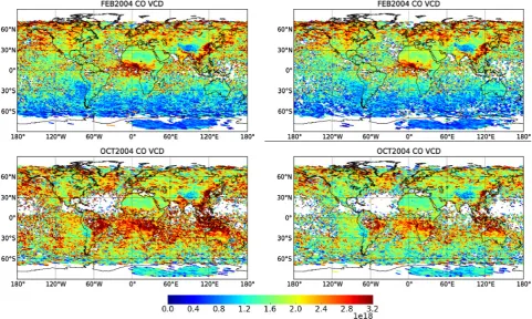
Since mission start, the number of dead/bad pixels has grown steadily, cf. Fig. 3a, and in June 2009 around 40 % of the pixels in channel 8 are marked as bad. Fig. 4 shows the effect on CO VCD retrievals of using a constant mask for one year vs. using a dynamic mask continuously updated Lichtenberg et al. (2010). Even though the total number of flagged pixels does not change dramatically between Febru-ary and October 2004, cf. Fig. 3b, the retrieved VCDs differ significantly, i.e. CO fits depend on the presence of the indi-vidual pixels and their quality. This result was already found earlier by Gloudemans et al. (2005) for CO retrievals with the IMLM algorithm.
3.3 Sensitivity to signal changes in individual pixels
An inversion process aims at gaining information about model parameters from observed quantities. In the case of atmospheric gas retrievals, the observed quantities are the ra-diances measured at different wavelengths for a light beam that has traveled through the Earth’s atmosphere. Since the absorption of light by atmospheric gas constituents is wavelength-dependent, the discrete measured radiance spec-trum contains implicit information of gas concentrations: the higher the concentration of moleculem, the lower the radi-ance at wavelengths where gasmabsorbs (see Sect. 2.1 for details).
In this subsection, the spectral sensitivity of the molecu-lar scaling factorsαmis studied by sequential perturbations on individual pixels of SCIAMACHY channel 8. On the one hand, a response of a molecular scaling factorαm to a per-turbation on a given spectral pixel means that this pixel con-tains information about the atmospheric content of molecule
mand that the inclusion of this pixel would be beneficial for the inversion. On the other hand, some radiative and spec-troscopic aspects such as the interference of spectral lines of the target gas with strong lines of other gases, or insufficient knowledge of molecular absorption cross sections due to im-precise spectral line parameters can lead to errors during the inversion process. Consequently, those critical pixels where perturbations have large impacts on several molecules at the same time should be treated with care.
A synthetic SCIAMACHY spectrum covering the whole channel (1004 pixels ignoring the blinded 20 pixels at the left and right ends) with a representative viewing geome-try was produced by means of GARLIC (the BIRRA for-ward model). An inversion of this unperturbed noise-free “reference” spectrum delivers scaling factors of unity for all gases. Gradually, the intensity spectrum was perturbed pixel by pixel by constant amounts:
Iijpert=(1+aj)×Iirefwithaj=0.1×j
fori=1,...,1004 andj= −10,...,10 (21) where the index idenotes the spectral pixel number andj
the perturbation. For instance,Ii,−10 represents a
perturba-tion on the ith pixel of−100 % (i.e. Ii,−10=0), Ii,0 is the
unperturbed reference radianceIiref, andIi,10a perturbation
of 100 % (i.e. 2Iiref).
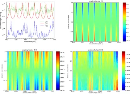
Figure 5 shows the results of this study around the CO fit-ting window (4282–4303 cm−1) in channel 8. The absorp-tion cross secabsorp-tions of CO, CH4, and H2O are depicted in
Fig. 5 (top left panel) for reference. Note that eight CO lines are shown, whereas only the central six are actually included
Fig. 4. Comparison of a retrieval using a constant mask flagging only pixels that are marked as “bad” for at least half of the cases of the year 2004 (left) and a retrieval using a dynamic mask appropriate for each measurement (right). In February (top) the results look similar while the result for October (bottom) is noisier for the constant mask that does not flag all bad pixels. CO VCD in units molec cm−2.
in the aforementioned fitting window. The further panels show the impact of the perturbations on the fitted molecular scaling factorsαCO,αCH4andαH2O. The patterns of the
ef-fect of pixel perturbations on the different gas retrievals look completely different, reflecting the structure of the cross sec-tions. Perturbations of pixels close to the center of strong absorption lines have mostly a large impact on the retrieved columns, whereas a perturbation on pixels far away in the wings does not alter significantly the retrievals. In absolute values, the effect is very different for CO (up to a factor 2) than for the other two gases (few percent). Both, water vapor and methane absorb substantially over the entire channel, so the perturbation of a single pixel is not critical. On the other hand, carbon monoxide has much weaker absorption lines and only in part of the channel, and consequently is more sensitive to the quality of the spectra. Indeed, some pertur-bations even resulted in negative CO scaling factors. Recall that for this sensitivity study, the measurement vectory com-prises 1004 elements. In case of the CO retrieval window, the size of the measurement vector is considerably reduced and the effect of radiance perturbations on theα’s increases significantly (orders of magnitude for CO), since individual pixels gain in relative weight. Note that for operational re-trievals the fitting window cannot cover the whole channel due to the timeliness requirements on data availability.
According to Fig. 5, the effect on H2O retrievals seems
to be small. However, water vapor is highly variable spa-tially and temporally, and the water profile assumed in the model has a strong impact on the retrieval result, cf. Fig. 6. Furthermore, molecular spectroscopy of water is quite del-icate and, according to Rothman et al. (2009), “the recom-mended line list for water remains in a state of constant evo-lution.” In laboratory spectroscopy, an accurate determina-tion of the amount of water in the absorpdetermina-tion cell is difficult, thus any error in the number density nleads to a system-atic error (over- or underestimate) of line strengths. For all 92 water lines in the 4280–4305 cm−1wavenumber interval,
HITRAN2008 gives an uncertainty range between 5 and 10 % for line strengths. Note that optical depthτ and transmission
T depend on the product of line strength and number density,
Sn(see Eqs. 3 and 4); moreover, in the lower atmosphere the line center value of the molecular absorption is proportional toSn/γLwhereγLis the Lorentz width. In conclusion, the
uncertainty of both, water density profile and water line pa-rameters suggests the omission of further pixels sensitive to water, i.e. those near strong H2O absorption lines possibly
Fig. 5. Sensitivity of BIRRA CO VCDs with respect to perturbations of individual pixels. Top left: absorption cross sections of CO (red), CH4(green dashed), and H2O (blue long dashed) in channel 8 CO fitting window. Other plots: molecular scaling factors as a function of
individual pixel perturbations. Note the different range of the color bars.
Fig. 6.
Comparison of two VCD
[molec
/
cm
2]
retrievals for February 2004. Left: all good pixels
in the retrieval window are used. Right: pixels over lines with strong water vapour interference
are excluded. In the latter case several features like enhanced CO values in South-East Asia
and the North-South gradient are more clearly visible.
and number density,
Sn
(see Eqs.
(3)
and
(4)
); moreover, in the lower atmosphere the
line center value of the molecular absorption is proportional to
Sn/γ
Lwhere
γ
Lis the
Lorentz width. In conclusion, the uncertainty of both water density profile and water
line parameters suggests the omission of further pixels sensitive to water, i.e. those
near strong
H
2O
absorption lines possibly not modeled sufficiently well.
3.4
Ice layer and instrument transmission
The NIR detectors of SCIAMACHY are the coldest point of the instrument. Since not
all water was removed from ENVISAT during the commissioning phase, an ice layer
is deposited on the detector surface (this layer is regularly removed by heating the
detectors). The ice reduces the transmission in a wavelength dependent way;
further-more it scatters the incoming light and generally leads to a broadening of the spectrum
(Lichtenberg et al., 2006; Gloudemans et al., 2005). To account for this effect in carbon
monoxide retrievals from channel 8 spectra, BIRRA treats the slit function width
γ
Gas
23
Fig. 6. Comparison of two VCD [molec cm−2] retrievals for February 2004. Left: all good pixels in the retrieval window are used. Right: pix-els over lines with strong water vapour interference are excluded. In the latter case, several features like enhanced CO values in South-East Asia and the North-South gradient are more clearly visible.
3.4 Ice layer and instrument transmission
The NIR detectors of SCIAMACHY are the coldest point of the instrument. Since not all water was removed from ENVISAT during the commissioning phase, an ice layer is deposited on the detector surface (this layer is regularly re-moved by heating the detectors). The ice reduces the
trans-mission in a wavelength dependent way; furthermore it scat-ters the incoming light and generally leads to a broadening of the spectrum (Lichtenberg et al., 2006; Gloudemans et al., 2005). To account for this effect in carbon monoxide re-trievals from channel 8 spectra, BIRRA treats the slit func-tion HWHMγas an additional auxiliary fit parameter.
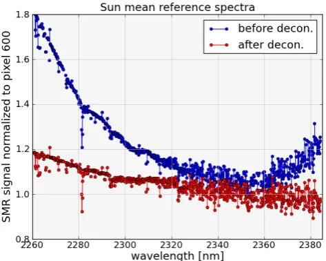
Fig. 7.Sun mean reference (SMR) spectrum in channel 8 with ice layer (blue) and with clean detector (red), normalised to the signal in an arbitrary pixel to illustrate the change in the spec-tral shape.
24
Fig. 7. Sun mean reference (SMR) spectrum in channel 8 with ice layer (blue) and with clean detector (red), normalised to the signal in an arbitrary pixel to illustrate the change in the spectral shape.
Figure 7 shows a typical sun mean reference (SMR) spec-trum shortly after decontamination, i.e. with only a thin or no ice layer and a SMR spectrum several weeks later. The change of the spectral shape due to the ice extinction is clearly visible. See also Subsect. 4.1 for a discussion about the impact of the ice layer on mean instrument transmittance or throughput.
3.5 Solar spectrum
The solar irradiance spectrum used in the radiative transfer model, Eq. (10), also has some impact on the retrieval prod-uct. BIRRA can use the SMR spectrum measured daily (as an average of a series of measurements) by SCIAMACHY for calibration and scientific purposes. Alternatively, a va-riety of solar spectra models and measurements is available (e.g. Abrams et al., 1996; Hase et al., 2006), and BIRRA can read solar irradiance spectra of Kurucz (1995) (extracted from MODTRAN4, Berk et al., 1999).
Figure 8 illustrates relative differences of some selected fit parameters when using, on the one hand, the Kurucz model solar spectrum and the SCIAMACHY SMR spectrum, on the other hand. The first row shows relative differences for the CO scaling factorαCO, the second row for the CH4scaling
factorαCH4 and the third row for xCO column density. The
left column shows the results of the month February 2004 whereas the second one presents those of July 2004. Red-dish color (indicating higher values of the fit values for the Kurucz spectrum compared to the SMR spectrum) dominates in all plots of Fig. 8 with no exception, i.e. the use of the Ku-rucz spectrum biasesαCO,αCH4 and xCO to higher values.
Note, however, that the color bar ofαCH4ranges from−0.1
to 0.1 (±10 %), whereas that of αCO and xCO ranges from
−0.5 to 0.5 (±50 %). Thus, the impact of the solar spectrum is much higher on CO than on CH4. The difference
distri-butions ofαCH4 are quite homogeneous, with the exception
of the Tibetan Plateau and the Andes Cordillera, where the differences increase. The distributions ofαCOand xCO are
very similar indicating that the effect of the solar spectrum on xCO is caused basically by the effect of the solar spectrum onαCOrather than onαCH4. The CO difference distributions
show latitude (solar zenith angle) as well as seasonal depen-dency (the pattern in February and July differ considerably). Since SMR and Earth’s spectra are measured with the same detector, most artificial features are included in both spectra. This is an advantage of SCIAMACHY’s SMR spec-trum with respect to Kurucz or any other solar specspec-trum, since in the latter cases, artifacts in Earth’s spectra would be attributed by the model to atmospheric effects. As a consequence SCIAMACHY’s SMR spectra are used in the retrievals.
3.6 Spectral calibration
In order to ensure high spectral stability over the lifetime of the mission, SCIAMACHY has been equipped with a spec-tral calibration lamp, the “Specspec-tral Line Source” (SLS), for determining the pixel-to-wavelength relationship. Whereas the SLS has proved to be suitable for a precise in-flight spec-tral calibration of channels 1 to 6, it is not sufficient for the calibration of channel (7 and) 8 due to the lack of enough SLS spectral lines within these channels. Because of this, the pixel-to-wavelength relationship of channel 8 in the level-1b product is set to the ground calibration. Although on-ground calibration was performed under representative flight conditions (temperature and vacuum), a similar spectral tun-ing as in the other channels should be applied to channel 8 for a precise spectral calibration.
Information from molecular spectroscopy (as provided by the HITRANor GEISA database) can be exploited for spec-tral calibration, i.e. an in-flight specspec-tral calibration for the SCIAMACHY channel 8 can be performed utilizing absorp-tion signatures of atmospheric methane, water vapor and car-bon monoxide. The spectral correction found has roughly a second-degree polynomial dependency and its value can be as large as 0.5 nm (more than 4 pixels) at the right edge of channel 8, see Fig. 9. Within the CO fitting window, the spec-tral correction is well approximated by a first-degree polyno-mial, i.e. shift and squeeze.
Fig. 8. Influence of the solar spectrum on monthly average CO retrievals. The plots show relative differences ofαCO(top),αCH4(mid), and
xCO (bottom) of retrievals with the Kurucz solar spectrum vs. the SCIAMACHY SMR spectrum for two months in 2004: February (left) and July (right).
Fig. 9.Spectral correction to the on-ground pixel-to-wavelength relationship.
negatively biased VCD distributions (note the different color bars) and unrealistic re-gional patterns (e.g. Himalayas).
3.7 Spectroscopic input data: line parameters and continuum
Spectroscopic line parameter databases such as HITRAN(Rothman et al., 2009) or GEISA(Jacquinet-Husson et al., 2008) are an essential input for the computation of molecular cross sections (Eq. 4). Recently, Frankenberg et al. (2008a,b) have
dis-28
Fig. 9. Spectral correction to the on-ground pixel-to-wavelength relationship.
3.7 Spectroscopic input data: line parameters and continuum
Spectroscopic line parameter databases such as HITRAN
(Rothman et al., 2009) or GEISA (Jacquinet-Husson et al., 2008) are an essential input for the computation of molecular cross sections (Eq. 4). Recently, Frankenberg et al. (2008a,b) have discussed the importance of accurate and complete line parameters for methane retrievals in SCIAMACHY channel 6. In the short–wave end of SCIAMACHY channel 8, wa-ter vapor spectroscopic data are significantly different in the recent version of these databases. Feng and Zhao (2009) dis-cusses impacts of changes of the HITRAN database on near infrared transmittances, and in SCIAMACHY’s channel 8 found the most noticeable changes for wavenumbers larger than 4350 cm−1. In the middle of this channel used for CO retrievals, there are only minor changes, and the retrievals do not show a strong impact.
The default setting for the retrieval of CO column densi-ties from SCIAMACHY channel 8 considers three absorbers, i.e. CO, CH4, and H2O. Although there are no CO2lines in
the center of channel 8, there is a contribution of a small, yet
Fig. 10. Comparison of xCO retrievals without (left) and with wavenumber calibration. Note the different color bar with xCO values ranging down to−3·1018molec cm−2for the unshifted wavenumber retrievals (left). (DBPM provided by M. Buchwitz, personal communication, October 2006).
non-vanishing CO2continuum. However, adding CO2as an
additional absorber has a negligible effect on the retrieved xCO product.
3.8 Atmospheric input data
VCDs are retrieved in BIRRA by fitting the scaling factors
αmof concentration profilesnm(z)(see Eqs. 1, 8). Accord-ingly, the quality of the retrieval clearly depends on the ad-equacy of the profiles used. Furthermore, pressure and tem-perature data are required to evaluate the molecular cross sectionsk(ν,p,T )in Eq. (4). Test retrievals for orbit 8663 using the six AFGL model atmospheres (Anderson et al., 1986) reveal that the fitted CO column densities are espe-cially sensitive to temperature.
Clearly, the use of just a few atmospheric profiles (as pro-vided by the AFGL data) does not really cover the full sea-sonal and spatial variability. There are different strategies to better represent the atmospheric state in the retrievals: Buch-witz et al. (2004) use a single profile of temperature, pres-sure, and trace gas mixing ratios from the US Standard at-mosphere (with methane scaled to 1750 ppbv), and fits an additional temperature shift parameter to account for the tem-perature dependence of the molecular absorption cross sec-tions. In Gloudemans et al. (2008), temperature and H2O
profiles are taken from the European Centre for Medium-Range Weather Forecasts (ECMWF).
Because molecular cross sections are computationally ex-pensive and operational processing imposes timeliness con-straints, BIRRA uses a compromise and takes a single pres-sure and temperature profile for each state selected from the CIRA-86 data base according to time and mean latitude. The Committee on Space Research (COSPAR) International Ref-erence Atmosphere (CIRA) provides monthly mean profiles of pressure vs. temperature for the altitude range 0–120 km with almost global coverage (80◦N–80◦S) (Fleming et al.,
1990, http://badc.nerc.ac.uk/data/cira/). Trace gas profiles are taken from the US Standard Atmosphere.
3.9 Least squares settings
Solvers for nonlinear least squares problems usually offer several input parameters to control the iterations. In addi-tion to terminaaddi-tion code due to excessively large number of iterations, the PORT library delivers convergence codes for standardx–tolerance (relative change of the norm of thex
state vector) andy–tolerance (relative change of the norm of the residual vectory−F (x)) (Gay, 1990). In our applica-tions, “relative function convergence” was reached for most of the cases.
Ideally, the different least squares solvers provided by PORT should give identical retrieval results. Figure 11a shows that the retrieved carbon monoxide VCDs (averaged within a 1 dg latitude belt over all longitudes) of orbit 8663 (27 October 2003) are very similar for all methods. Differ-ences can be expected for “difficult” observations, i.e. when the fit did not converge properly or some of the fitted pa-rameters are exceptionally small or large. Especially in case where the iterative optimization algorithm suggests a step leading to one or several negative fit variables, differences show up in the constrained and unconstrained retrievals. In fact, the spikes around 20◦N and 32◦S do not show up in both constrained least squares results. Various strategies have been discussed, how an algorithm should proceed when some of the physical variables reach “forbidden” (usually negative) values; common approaches are to stop the iterative solution process, or to ignore and continue (and accounted for in the post-processing of the data). In case of unconstrained least squares fits, BIRRA stops the iteration when it encounters negative slit function widths or in case of too many negative scaling factors.
distributions of carbon gas vertical column densities. In the following subsections, a survey of BIRRA carbon monoxide retrieval results is given, followed by a brief presentation of first BIRRA methane retrievals.
4.1 Monitoring of fit parameters
In the previous subsections, the impact of the level 1b data quality on carbon monoxide retrievals has been discussed. Fig. 12 and 13 illustrate time series of the fit parameters for CO retrievals in channel 8. The panels of Fig. 12 show, from top to bottom, the mean channel transmission (throughput), the scaling factors of CO, CH4and H2O, the HWHM of the
instrument slit function, and the zeroth, first, and second de-gree coefficients of the albedo polynomial. Although the throughput is not a fit parameter, it has been included here for comparison. Because of the difficulty in modeling the ice layer on top of channel 8, it has an impact on the fitted parameters.
Since the ice layer reduces the mean intensity, the through-put (the mean instrument transmission) is a good indicator of its thickness. Table 1 shows the cross-correlationρ of the different fit parameters with respect to the throughput. Note that these coefficients are calculated for the 14-days averaged time series, not for individual observations. They are nor-malized between−1 (full anti-correlation) and 1 (full cor-relation). A high correlation coefficient (in absolute value) means that the two curves follow a similar course and it will be taken here as evidence for a possible causal relationship. Table 1 illustrates that (the scaling factor of) CH4is the most
affected parameter by the ice layer growth. The second de-gree polynomial coefficient r2 has the second highest
cor-relation, suggesting that the normalization of the observed spectra by the SMR spectrum does not completely elimi-nate the change in spectral shape due to scattering in the ice layer. These conclusions are backed by Fig. 12. Accord-ing to Tab. 1, the first degree polynomial parameter (r1), the
HWHM and CO are less affected by the ice layer. A detailed examination of the curves in Fig. 12, however, shows that
r1does have a strong anti-correlation with the throughput,
but two outliers lower the value of ρ. Remarkably, ther0
accordingly.
The time series in Fig. 13 show a general trend of increas-ing fit errors indicatincreas-ing that the results become continuously worse. Since the model remains the same, this can only be interpreted as a decrease of the measurement quality. The curves also show some time intervals with exceptionally high errors, e.g. June 2006 and 2007, most likely due to the incor-poration of some bad pixels in the fit.
4.2 Carbon monoxide
Carbon monoxide is an important trace gas affecting air qual-ity and climate. Although CO is not considered as a green-house gas, it is relevant as a precursor for carbon dioxide. CO is also one of the major precursors of tropospheric ozone. It is highly variable in space and time. In the troposphere, about half of the CO originates from anthropogenic sources (e.g. fossil fuel combustion), and further significant contri-butions are due to biomass burning. With its photochemical lifetime of one to three months, CO is a good tracer of trans-port in the troposphere as well as in the strato– and meso-sphere.
With passive atmospheric remote sensing, carbon mono-xide can be observed in several spectral regions from the microwave to the near infrared. CO is a target species of several spaceborne instruments, nb. AIRS (McMillan et al., 2005, 2008), MOPITT (Deeter et al., 2003, 2009), and TES (Rinsland et al., 2006) from NASA’s nadir sounders aboard the EOS satellite series; MIPAS and SCIAMACHY on ESA’s Envisat, and more recently it has also been observed by IASI on MetOp (Fortems-Cheiney et al., 2009; George et al., 2009; Illingworth et al., 2011).
4.2.1 Retrieval errors
The error of the proxy normalized VCD, Eq. (1), is estimated from the errors of the column scaling factorsαCOandαCH4,
that, in turn, are obtained from the diagonal elements of the least squares covariance matrix defined by
4=σ2JTJ −1
with σ2= ky−F(x)k2/(m−n)
−40 −20 0 20 40 60 Latitude [dg]
0 2 4 6
xCO [10
18 molec/cm 2 ]
n2g n2gb nsg nsgb
0 1 2 3 4
xCO (n2g) 0
1 2 3 4
xCO (nsg)
y = 1.019x − 1.165e16
correlation coeff. 0.9963
Fig. 11.Sensitivity of CO retrievals with respect to least squares algorithm for orbit 8663 (27. October 2003, covering Russia, the Arabic peninsula, and Eastern Africa): a) Comparison of CH4-normalizedCOvertical columns (xCO). “n2g” and “nsg” denotes nonlinear and separable
least squares, respectively; “b” indicates the bound constrained versions. b) Scatter plot of xCO retrieved using nonlinear least squares (“n2g”, horizontal axis) vs. separable least squares (“nsg”, vertical axis).
32
Fig. 11. Sensitivity of CO retrievals with respect to least squares algorithm for orbit 8663 (27 October 2003, covering Russia, the Arabic peninsula, and Eastern Africa): (a) comparison of CH4-normalized CO vertical columns (xCO). “n2g” and “nsg” denote nonlinear and
separable least squares, respectively; “b” indicates the bound constrained versions. (b) Scatter plot of xCO retrieved using nonlinear least squares (“n2g”, horizontal axis) vs. separable least squares (“nsg”, vertical axis).
Table 1. Cross correlation coefficientsρbetween fit parameters and throughput.
parameter CO CH4 H2O HWHM refl0 refl1 refl2
correlation with throughput 0.374 0.701 0.044 −0.399 0.257 −0.401 0.526
whereJ denotes the Jacobian (Gay, 1990). Note that the scaled residual normσ2contains both, errors due to instru-mental noise and deficiencies of the forward model.
Since the spectral information on carbon monoxide in the observed spectrum is small, the retrievals are specially sensi-tive to instrumental noise. The signal-to-noise ratio depends on the surface (or cloud) albedo and solar irradiance (essen-tially SZA), hence dark areas and high latitudes are expected to have higher retrieval errors. Since in most of the cases the CO information is comparable or even lies under the noise level, the precision of the individual estimates is low and it is customary to deliver the CO retrievals as spatial and temporal averages on a regular longitude/latitude grid.
Deficiencies of the forward model introduce systematic er-rors to the CO estimates. One of the major assumptions in BIRRA is the neglect of scattering within the atmosphere. Homogeneous aerosol and cloud (e.g. low marine stratocu-muli) layers are satisfactorily accounted for by proxy mod-eling. However, under highly convective conditions, cloud heterogeneity can cause large retrieval errors.
Fig. 12.
Time series of 14-day averaged fit parameters included in CO retrievals in channel 8.
From top down: the mean channel transmission (throughput), the scaling factors of
CO
,
CH
4and
H
2O
, the half width at half maximum of the instrument slit function, and the zeroth, first, and
second degree coefficients of the albedo polynomial. See the dependency of some parameters
on throughput.
35
Fig. 12. Time series of 14-day averaged fit parameters included in CO retrievals from channel 8. From top down: the mean channel transmission (throughput), the scaling factors of CO, CH4and H2O, the half width at half maximum of the instrument slit function, and the
zeroth, first, and second degree coefficients of the albedo polynomial. See the dependency of some parameters on throughput.
over the Indian Ocean and West Equatorial Pacific during the Asian Monsoon period (from June to September, see bottom left summer panel in Fig. 14). Accordingly, only few obser-vations pass the quality filter, see Fig. 15.
The histograms in Fig. 16 illustrate the occurrence fre-quency of xCO errors, i.e. the unnormalized error probabil-ity densprobabil-ity function (PDF). The errors are slightly higher in summer (right panel) than in winter (left panel), which is re-flected by the median values and in accordance with Fig. 14.
4.2.2 Spatial distributions
CO vertical columns have been processed for several years from 2003 to 2009 using the BIRRA algorithm and a dy-namic bad & dead pixel mask (see Subsect. 3.2). Figure 17 shows the annual mean of CO vertical columns for the years 2003, 2004, and 2005. In addition to the selection criteria mentioned in Sect. 2.3, the relative errors of retrievals (er-rors ofαCOless than 50 %, error ofαCH4less than 1 %) are
Fig. 13.
Time series of 14-day averaged errors of fit parameters (see Fig. 12). From top down:
error of the scaling factors of
CO
,
CH
4and
H
2O
, the half width at half maximum of the instrument
slit function, and the zeroth, first, and second degree coefficients of the albedo polynomial.
36
Fig. 13. Time series of 14-day averaged errors of fit parameters (see Fig. 12). From top down: error of the scaling factors of CO, CH4
and H2O, the half width at half maximum of the instrument slit function, and the zeroth, first, and second degree coefficients of the albedo
polynomial.
taken into account. All annual averages show high densi-ties at South East Asia due to anthropogenic emissions and in Central Africa due to high density of biomass burnings during the dry seasons. It can be also noticed that the CO column densities were specially high during 2003. This CO increase in 2003 is related to the increase in biomass burnings during this year, and has also been reported by other studies (e.g. Buchwitz et al., 2007).
Figure 18 provides a closer look to the African continent. In this case, the results are presented as a three year aver-age of the four seasons. Inter-tropical regions are the ar-eas showing higher sar-easonality. The weather in the ical region of the Earth is highly influenced by the trop-ical rain belt, which oscillates between the Northern and
Southern Hemisphere. In the Northern Hemisphere, the wet season comprises roughly the months from April to Septem-ber, whereas the dry season lasts from October to March. Due to the rain bell oscillation, in the Southern Hemisphere the wet and dry seasons are reverted. During the dry sea-son, biomass burning events are more likely to occur. The seasonality of the fires can be clearly seen in the carbon monoxide distributions: the inter-tropical regions present the highest CO VCDs at the end of the dry seasons (January-February-March in the northern and July-August-September in the Southern Hemisphere).
Fig. 14.
XCO mean errors
[
molec
/
cm
2]
averaged over the four seasons 2003 – 2005.
Top-left: December-January-February, top-right: March-April-May, bottom-Top-left: June-July-August,
bottom-right: September-October-November.
39
Fig. 14. xCO mean errors [molec cm−2] averaged over the four seasons 2003–2005. Top-left: December-January-February, top-right: March-April-May, bottom-left: June-July-August, bottom-right: September-October-November.
Fig. 15.
Number of observations accepted for carbon monoxide vertical columnn densities
retrievals, seasonal three-year averages. (Arrangement as in Fig. 14)
account. All annual averages show high densities at South East Asia due to
anthro-pogenic emissions and in Central Africa due to high density of biomass burnings during
the dry seasons. It can be also noticed that the CO column densities where specially
high during 2003. This CO increase in 2003 is related to the increase in biomass
burn-ings during this year, and has also been reported by other studies (e.g. Buchwitz et al.
(2007)).
Fig. 18 provides a closer look to the African continent. In this case, the results
are presented as a three year average of the four seasons. Inter-tropical regions are
40
Fig. 15. Number of observations accepted for carbon monoxide VCD retrievals, seasonal three-year averages (arrangement as in Fig. 14).
Fig. 16. Histograms of carbon monoxide vertical column density errors, three-year (2003 – 2005) seasonal averages. Left: winter; right: summer.
the areas showing higher seasonality. The weather in the tropical region of the Earth
is highly influenced by the tropical rain belt, which oscillates between northern and
southern hemisphere. In the northern hemisphere, the wet season comprises roughly
the months from April to September, whereas the dry season goes from October to
March. Due to the rain bell oscillation, in the southern hemisphere the wet and dry
seasons are reverted. During the dry season, biomass burning events are more likely
to occur. The seasonality of the fires can be clearly seen in the carbon monoxide
distributions: the inter-tropical regions present the highest CO VCDs at the end of the
dry seasons (January–February–March in the northern and July–August–September
in the southern hemisphere).
Fig. 19 illustrates the three-year average of xCO over Southeastern Asia. Regions
with a high population density such as the Sichuan Basin (Red Basin) in South-West
China or the Chinese eastern coast area are clearly visible with a high carbon
mono-xide abundance, as was already observed by, e.g. SCIAMACHY (Buchwitz et al., 2006;
41
Fig. 16. Histograms of carbon monoxide vertical column density errors, three-year (2003–2005) seasonal averages. Left: win-ter; right: summer.
Fig. 17.
Annual mean carbon monoxide
vertical column densities
[
molec
/
cm
2]
for
2003 to 2005. (
1
◦×
1
◦grid with
3
◦×
3
◦me-dian filter smoothing)
42
Fig. 17.
Annual mean carbon monoxide
vertical column densities
[
molec
/
cm
2]
for
2003 to 2005. (
1
◦×
1
◦grid with
3
◦×
3
◦me-dian filter smoothing)
42
Fig. 17. Annual mean carbon monoxide vertical column densities [molec cm−2] for 2003 to 2005. (1◦×1◦grid with 3◦×3◦median filter smoothing)
China or the Chinese eastern coast area are clearly visible with a high carbon monoxide abundance, as was al-ready observed by, e.g. SCIAMACHY (Buchwitz et al., 2006; Gloudemans et al., 2009) and the MOPITT mission (Clerbaux et al., 2008).
4.2.3 Intercomparison with ground-based observations
Fig. 18.
Three year averages (2003 – 2005) of quarterly mean CO VCDs
[molec
/
cm
2]
over
Africa. From top-left to bottom-right: January-February-March, April-May-June,
July-August-September, and October-November-December.
(
0
.
2
◦×
0
.
2
◦grid with
1
◦×
1
◦median filter
smoothing)
43
Fig. 18. Three year averages (2003–2005) of quarterly mean CO VCDs [molec cm−2] over Africa. From top-left to bottom-right: January-February-March, April-May-June, July-August-September, and October-November-December. (0.2◦×0.2◦grid with 1◦×1◦median filter smoothing)
Fig. 19.Three-year average ofCOvertical column densities[molec/cm2]over South-East Asia. (0.2◦×0.2◦grid with1◦×1◦median filter smoothing)
Gloudemans et al., 2009) and the MOPITT mission (Clerbaux et al., 2008).
44
Fig. 19. Three-year average of CO vertical column densities [molec cm−2] over South-East Asia. (0.2◦×0.2◦grid with 1◦×1◦ median filter smoothing).
Dils et al. (2006) described comparisons between SCIA-MACHY CO, CH4, CO2, and N2O total columns retrieved
by three different algorithms (WFM-DOAS, Buchwitz et al., 2004; IMAP-DOAS, Frankenberg et al., 2005a; and IMLM, de Laat et al., 2006) and ground-based FTIR data mea-sured at eleven NDACC (then NDSC) stations. More re-cently, de Laat et al. (2010) reported good agreement be-tween SCIAMACHY IMLM retrievals of carbon monoxide with twenty ground-based stations (mostly FTIR).
These intercomparisons are delicate since the instruments have different altitude sensitivity and horizontal resolution, the temporal match of the observations is not ideal and the lo-cation of the ground stations and the surrounding terrain may also be an impediment. Nevertheless, these studies allow an assessment of, e.g. relative biases or inter-annual variability and are an important element of the validation efforts.
Satellites observe large areas in contrast to the point-like view of uplooking ground-based spectrometers, so they see
in general a larger portion of the atmosphere. If compar-isons were performed over a largely uniform surface terrain without emission sources, the problem of the horizontal res-olution would be reduced. Accordingly, oceans are natural candidates but, in the absence of clouds, the signal received is rather weak because of the low albedo of water (see also Gloudemans et al., 2009). Another possibility is to use desert areas without significant emissions. Although deserts can exhibit altitude differences, they typically have high surface albedos providing high signal-to-noise ratios.
Here, SCIAMACHY CO BIRRA retrievals are compared to the ground-based measurements provided by the World Data Center for Greenhouse Gases (WDCGG) Assekrem Station (Novelli et al., 2003). It is important to note at this point that the SCIAMACHY CO retrievals represent (dry-air) column mixing ratios (i.e. considering the a-priori col-umn mixing ratioqCOprior instead of the a-priori vertical col-umn densityNCOprior in Eq. (19)), whereas the Assekrem sta-tion measured volume mixing ratios at surface level. Such a comparison is only justified for gases with constant mixing ratio profiles (e.g. O2, CO2) and this is not the case of CO.
This study in not intended to be a validation, since we are comparing two different quantities. However, both retrievals should show similar seasonality features and temporal evolu-tion (and indeed they do) and this is our motivaevolu-tion here.
Figure 20 illustrates time series of 14-day averaged dry-air CO column mixing ratios as observed by SCIAMACHY and CO volume mixing ratios as measured at the Assekrem WD-CGG ground station. In the Northern Hemisphere, higher column densities can be expected in winter, and this can be clearly seen in Fig. 20. Furthermore, the seasonal variation of carbon monoxide retrieved with BIRRA is also evident in the ground-based measurements. A good agreement of SCIA-MACHY’s and the Assekrem ground station CO is found for the years of 2003, 2004 and 2005. Afterward, due to in-strument degradation, the SCIAMACHY CO shows a higher dispersion and the seasonal variation is worse represented (esp. in 2006).
4.3 Methane
Methane is the third (second anthropogenic) most important greenhouse gas representing one fifth of the whole radiative forcing of long-life well-mixed gases. Its concentration has increased by more than a factor of two since pre-industrial times with a growth rate of about 1 % per annum (until re-cently). Atmospheric methane results from anthropogenic (agriculture, fossil fuel combustion, . . . ) as well as natu-ral (e.g. wetlands, geological processes) sources. With a life time of about ten years, its spatial and temporal variation is considerably smaller than for CO. As a consequence, the required retrieval precision is much higher.
Atmospheric sounding of methane is performed in the near and thermal infrared, and it is observed by all sensors mentioned above (e.g. Buchwitz et al., 2005; Frankenberg
Fig. 20.SCIAMACHY CO over Central Sahara and intercomparison with Assekrem WDCGG station data (Ahaggar Mountains, 2710 m above sea level). Note that the SCIAMACHY CO retrievals are dry-air column mixing ratios and the Assekrem WDCGG CO data are volume mixing ratios at surface level. The time step is in both cases 14 days. The error bars represent the standard deviation of the data.
47
Fig. 20. Intercomparison of SCIAMACHY CO over Central Sa-hara with Assekrem WDCGG station (Ahaggar Mountains, 2710 m above sea level) data. Note that the SCIAMACHY CO retrievals are dry-air column mixing ratios and the Assekrem WDCGG CO data are volume mixing ratios at surface level. The time step is in both cases 14 days. The error bars represent the standard deviation of the data.
et al., 2006; Gloudemans et al., 2008). Furthermore, it is one of the two target gases of the TANSO Fourier trans-form spectrometer on-board the recently launched GOSAT satellite (Kuze et al., 2009).
For methane retrievals from SCIAMACHY observa-tions, two microwindows in channel 6 are utilized: the 5986–6139cm−1 interval with CH4 as the strongest
ab-sorber, and the 6273–6419cm−1 interval with CO2 as the
strongest absorber. For our retrievals, H2O has been
consid-ered as additional absorber in both windows, the Gaussian slit function HWHM has been fixed to 2.45 and 2.64cm−1
in the two windows, and albedo was modeled as a second degree polynomial.
Figure 21 gives an impression of three month averages for 2004. Regions of strong emissions, e.g. the northern South America, the equatorial region of Africa, and in Asia are clearly visible and reflect patterns found by, e.g. Frankenberg et al. (2006); Schneising et al. (2009). Seasonal variability such as increased emissions in South East Asia due to rice cultivation is evident especially for July-August-September. Furthermore, the plot shows the shift of methane emissions over wetlands from southern to northern Africa and back.
5 Summary and outlook
Fig. 21. Quarterly means of methane [ppm] for 2004. In view of the reduced signal over oceans, onlyCH4over land is plotted. (2◦×2◦grid)
49
Fig. 21. Quarterly means of methane [ppm] for 2004. In view of the reduced signal over oceans, only CH4over land is plotted. (2◦×2◦
grid)
flexibility and precision, BIRRA is also a suitable tool for scientific investigations.
The fundamentals of the algorithm have been presented in Sect. 2. BIRRA analyzes radiance spectra instead of optical thicknesses (as in DOAS-like algorithms), since instruments measure the convolved radiance rather than the convolved optical thickness.
The inversion is done by standard nonlinear least squares or by separable least squares solvers, where linear and non-linear parameters are treated separately. Further distinctive features of the code are the optional use of bound constrained least squares, exact analytical derivatives by automatic dif-ferentiation, and “on demand” line-by-line computation of molecular cross sections.
The results presented here are dry-air quantities: vertical column densities in case of CO, with CH4 as proxy; and
dry-air column mixing ratios in case of CH4, with CO2 as
proxy. Whereas CO2is a good proxy for the dry air mass of
the observations, CH4has some deficiencies (much stronger
spectral signatures than CO, spatial variability, non-constant profile, etc). However, due to the much greater variability of CO, CH4can be used as an appropriate proxy.
Several aspects of the level 1 data have been investigated. It turned out that the effect of the dead/bad pixel mask (DBPM) has a major impact on the retrievals. In addition to masking spectral pixels with doubtful level 1 quality, one has
to consider further masking due to spectroscopic aspects; in particular, interference of spectral lines of the target gas with strong lines of other gases, or insufficient knowledge of the molecular cross sections due to imprecise spectral line pa-rameters. The use of radiance spectra normalized by sun mean reference (SMR) spectra helps reducing the impact of the ice layer over the detector on the retrievals. However, in case of BIRRA, the ice layer affects CO and CH4differently
and further treatment is needed. The pixel-to-wavelength re-lationship of channel 8 in SCIAMACHY level-1b product is set to the on-ground calibration and a spectral correction is needed. We found that the required spectral correction has roughly a second-degree polynomial shape that can be well approximated by a first-degree polynomial in the CO fitting window.
A survey of carbon monoxide and methane VCD retrievals has been presented with emphasis on the years 2003 to 2005. “Pre-” and “postprocessing” of the data turned out to be cru-cial, i.e. careful preparation of the level 1b data used as in-put to the least squares fitting and a meticulous examination of the fitted column density scaling factors for the genera-tion of scientific products is mandatory. In addigenera-tion, the final product is highly sensitive to the correct filtering of dubi-ous retrievals and to the appropriate consideration of scene cloudiness. Moreover, careful analysis of the time series of all fit parameters with respect to the instrumental mean
transmittance provides valuable hints for the postprocess-ing. Preliminary work exploiting SCIAMACHY’s channel 6 shows BIRRA’s potential for methane (and carbon dioxide) retrievals.
The further development of BIRRA is motivated by its dual role as an operational processor and a scientific tool. For the “scientific prototype”, we are currently working on an optimization and fine-tuning of the multiwindow fitting (required for methane and carbon dioxide retrievals). Fur-thermore, a better climatology esp. of temperature and wa-ter would be beneficial and likewise the treatment of clouds and aerosols can be improved in the forward model and/or in the post-processing. Finally, our verification and vali-dation efforts will be intensified, e.g. by intercomparisons with ground-based observations (NDACC-TCCON) as well as thermal infrared sounders such as AIRS, GOSAT, IASI, MOPITT, and TES (Schreier et al., 2010). Clearly, the lessons learned from the scientific analysis will be a valu-able guide for the ongoing upgrade of the operational proces-sor. The further refinement will allow a better analysis of the years 2006 and beyond that are even more challenging due to the continuous channel degradation, nb. increasing num-ber of bad or dead pixels.
Acknowledgements. Numerous discussions in the SADDU working group (esp. with Michael Buchwitz and Heinrich Bovens-mann, University Bremen; and Annemieke Gloudemans, Hans Schrijver, and Christian Frankenberg, SRON) are gratefully acknowledged. In particular we thank Michael Buchwitz for providing SCIAMACHY level 1, the channel 8 DBPM, and level 2 (WFM-DOAS) data, http://www.iup.uni-bremen.de/sciamachy/ NIR NADIR WFM DOAS/; Annemieke Gloudemans and Hans Schrijver kindly provided their SCIAMACHY carbon monoxide total column data. Data of ground-based CO measurements were downloaded from the World Data Centre for Greenhouse Gases (WDCGG) at http://gaw.kishou.go.jp/wdcgg/wdcgg.html. Finally we would like to thank our colleagues Adrian Doicu, Michael Hess, Thomas Trautmann, and Mayte Vasquez for stimulating discussions and Bernd Aberle, Klaus Kretschel, and Markus Meringer for computational support.
Edited by: P. K. Bhartia
References
Abrams, M. C., Goldman, A., Gunson, M. R., Rinsland, C. P., and Zander, R.: O
![Fig. 1.Jacobians [erg/s/(cm2srcm−1)/ppm] for molecular con-centration profile retrieval in channel 8: CO (top), CH4 (mid), andH2O (bottom)](https://thumb-us.123doks.com/thumbv2/123dok_us/197014.1513226/4.595.297.549.80.623/fig-jacobians-molecular-centration-prole-retrieval-channel-andh.webp)