www.the-cryosphere.net/8/1239/2014/ doi:10.5194/tc-8-1239-2014
© Author(s) 2014. CC Attribution 3.0 License.
Parameterization of basal friction near grounding lines in a
one-dimensional ice sheet model
G. R. Leguy1,2, X. S. Asay-Davis2,3,4, and W. H. Lipscomb2
1New Mexico Institute of Mining and Technology, 801 Leroy Place, Socorro, New Mexico 87501, USA
2Los Alamos National Laboratory, Los Alamos, New Mexico 87545, USA
3Courant Institute of Mathematical Sciences, New York University, 251 Mercer Street, New York, New York 10012-1185, USA
4Potsdam Institute for Climate Impact Research, Telegraphenberg A 31, 14473 Potsdam, Germany Correspondence to: G. R. Leguy ([email protected])
Received: 4 December 2013 – Published in The Cryosphere Discuss.: 14 January 2014 Revised: 16 May 2014 – Accepted: 5 June 2014 – Published: 18 July 2014
Abstract. Ice sheets and ice shelves are linked by the transi-tion zone, the region where flow dominated by vertical shear stress makes a transition to flow dominated by extensional stress. Adequate resolution of the transition zone is necessary for numerically accurate ice sheet–ice shelf simulations. The required resolution depends on how the basal physics is pa-rameterized. We propose a new, simple parameterization of the effective pressure near the grounding line, combined with an existing friction law linking effective pressure to basal stress and sliding, in a one-dimensional, fixed-grid, vertically integrated model. This parameterization represents connec-tivity between the basal hydrological system and the ocean in the transition zone. Our model produces a smooth transition between finite basal friction in the ice sheet and zero basal friction in the ice shelf. In a set of experiments based on the Marine Ice Sheet Model Intercomparison Project (MISMIP), we show that with a smoother basal shear stress, the model yields accurate steady-state results at a fixed-grid resolution of∼1 km.
1 Introduction
Antarctica’s contribution to sea level rise has increased in the past decade. While the contribution of the East Antarc-tic Ice Sheet (EAIS) remains steady, mass loss from the West Antarctic Ice Sheet (WAIS) has more than doubled (Velicogna, 2009; Rignot et al., 2011). Theoretical models
suggest that marine ice sheets like WAIS are susceptible to instabilities when they lie on bedrock that slopes upward in the direction of ice flow (Weertman, 1974; Schoof, 2007a). If these instabilities are triggered, mass loss will accelerate, exacerbating future sea-level rise and potentially leading to WAIS collapse (Vaughan and Spouge, 2002; Joughin and Al-ley, 2011). For this reason it is important to understand the dynamic processes that drive ice sheets in the region.
ice-sheet flow dominated by vertical shear stress transitions to ice-shelf flow dominated by extensional stress) in order to obtain numerically accurate ice sheet–ice shelf simulations (Durand et al., 2009; Cornford et al., 2013).
Several studies have investigated the effects of differ-ent friction laws on ice dynamics using one-dimensional, depth-integrated models (Muszynski and Birchfield, 1987; MacAyeal, 1989; Schoof, 2007a). Vieli and Payne (2005) and Schoof (2007a) prescribed a discontinuous friction law across the grounding line where the ice loses contact with the bed. In these models the friction is nonzero in the ice sheet, but abruptly falls to zero at the grounding line. These models have the drawback that very high grid resolution near the grounding line is required for convergence. In mod-els with fixed grids, a tolerance of a few kilometers in the grounding-line location requires a resolution on the order of tens to hundreds of meters (Durand et al., 2009; Gladstone et al., 2010a, b; Cornford et al., 2013), which is computation-ally prohibitive for large-scale simulations. This requirement was confirmed by the Marine Ice Sheet Model Intercompar-ison Project (MISMIP, Pattyn et al., 2012) which used the same basal friction law as in Schoof (2007a). In this project, participants using a variety of fixed-grid models found that the errors in grounding-line position were unacceptably high (100 km or more) at resolutions that were computationally feasible in three-dimensional models (∼1 km).
One way to reduce the computational cost is to use adap-tive mesh refinement (Goldberg et al., 2009; Gladstone et al., 2010b; Cornford et al., 2013), i.e., to subdivide the hori-zontal mesh near features where high resolution is needed. Durand et al. (2009) investigated this approach in a Stokes model with the basal friction law of Schoof (2007a). They performed a set of experiments based on the MISMIP exper-iments with the goal of reaching steady state when using very high resolution near the grounding line. Even with grid res-olution of 30 m in the transition zone, they found differences in the grounding-line position over an advance-and-retreat cycle of∼2 km, whereas theoretical arguments predict that there should be no difference.
In order to reduce the need for high resolution near the grounding line, Pattyn et al. (2006) proposed a smooth basal-friction parameter that decays exponentially to zero as the ice flows across the grounding line into the ice shelf. This ap-proach gave promising results, as the transition zone could be partially resolved even at 12.5 km grid resolution. However, the model introduced an arbitrary length scale of exponen-tial decay, and the basal friction remained nonzero (though small) in the ice shelf. Gladstone et al. (2012) showed that the need for high resolution could also be relaxed by decreasing the value of the basal drag coefficient, the ice softness, chan-nel width (when buttressing is included in the model), or by steepening the slope of the bedrock topography. Pattyn et al. (2006) and Gladstone et al. (2010a) also showed that higher-order interpolation at the grounding line, where the grounded ice sheet meets the floating ice shelf, could greatly reduce the
error in the grounding-line position, implying convergence at coarser resolution.
In the case of rapidly sliding ice streams, basal resistance is controlled by the underlying water-laden plastic till (Tu-laczyk et al., 2000a, b; van der Wel et al., 2013). The presence of liquid water lowers the effective pressure at the ice base, leading to reduced basal friction (Tulaczyk et al., 2000b; Carter and Fricker, 2012; van der Wel et al., 2013), an ef-fect not accounted for in many ice sheet models. Recent observations confirm the existence of basal drainage chan-nels that connect subglacial lake systems (Wingham et al., 2006; Fricker et al., 2009). Some of these drainage systems are found near grounding lines (Fricker and Scambos, 2009; Carter and Fricker, 2012), meaning that they are likely to connect to the ocean (Le Brocq et al., 2013). In a detailed hy-drology/till model, van der Wel et al. (2013) found that sub-glacial conduits can extend to the grounding line if sufficient water is available from local melting and upstream transport. They concluded that the Kamb Ice Stream currently does not have conduit systems but that the Rutford Ice Stream is con-nected to the ocean via a permanent conduit system. Cuffey and Paterson (2010, p. 283) suggested that a free connec-tion between subglacial water and the ocean is likely near the grounding line, though not plausible at 50 or 100 km up-stream.
Several previous models have included the effect of basal water pressure or meltwater depth in their friction laws. Bueler and Brown (2009) assumed plastic flow with a yield stress proportional to the effective pressure N (the differ-ence between the ice overburden pressure and the basal water pressure). They parameterized basal water pressure as a lin-ear function of water depth, with a maximum value equal to 95 % of overburden pressure. Pimentel et al. (2010) used the friction law of Schoof (2005), which predicts a basal shear stress proportional toNin the limit of fast flow and smallN. They treated basal water pressure as a nonlinear function of water depth, capped at the overburden pressure. Martin et al. (2011) assumed plastic flow with a yield stress proportional toN, with basal water pressure prescribed to be 96 % of over-burden pressure under the marine portion of the Antarctic Ice Sheet (including close to grounding lines). This parameteri-zation reduced but did not eliminate the discontinuity in basal friction at the grounding line.
In this paper we propose a new treatment of effective pres-sure near the grounding line, combined with an established friction law (Schoof, 2005) linking basal stress and sliding to the effective pressure. In Sect. 2 we present our one-dimensional, vertically integrated flowline model, including the new parameterization. We also discuss mathematical lim-its of the basal friction law and the numerical methods used for our simulations. In Sect. 3 we show simulation results with different values of the effective-pressure parameter p for different bedrock topographies. In Sect. 4 we discuss the limitations of the model and the implications for future devel-opment of three-dimensional ice-sheet models. Sect. 5 sum-marizes the main results. A more detailed description of the numerical method is provided in Appendix C.
2 Model
The shallow-shelf flowline model presented in this paper, which is similar to the model of Schoof (2007a), is one-dimensional, symmetric and depth-integrated. It is intended to represent the motion of a transversely and vertically aver-aged ice stream. It includes the effect of three stress terms: the longitudinal stress (τl), the basal stress (τb), and the driv-ing stress (τd). The model neglects lateral shear (and there-fore buttressing) and vertical shear, and thus is best used to simulate fast-flowing ice streams. While additional physics would be required to model realistic ice sheets, our model is a simple, computationally efficient tool for idealized studies of grounding-line dynamics.
2.1 Model equations
The model consists of an equation for the evolution of ice thickness (conservation of mass) and a vertically integrated stress-balance equation:
Ht+(uH )x=a, (1)
(H τl)x−τb+τd=0, (2) where subscripts x and t denote partial derivatives (e.g., Ht≡∂H
∂t ). The ice thicknessH, ice velocityu, and other
im-portant model variables are defined in Table 1. Table 2 gives the value of the accumulation rateaand other model param-eters. The longitudinal stressτlis vertically averaged, so that H τlis the vertically integrated stress. Derivations of Eqs. (1) and (2) can be found in Muszynski and Birchfield (1987) and MacAyeal (1989). From Schoof (2007a), the longitudinal-and driving-stress terms are
(H τl)x= h
2A¯−1nH|ux|
1
n−1ux i
x, (3)
τd= −ρigH sx. (4)
In Eq. (3), the stressτlincludes the nonlinear viscosity given by Glen’s flow law, whereA¯is the depth-averaged ice soft-ness andnis the Glen’s flow exponent. In Eq. (4),τdis the
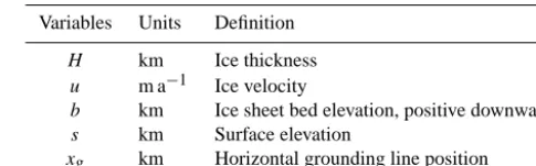
Table 1. Model variables.
Variables Units Definition
H km Ice thickness
u m a−1 Ice velocity
b km Ice sheet bed elevation, positive downward
s km Surface elevation
xg km Horizontal grounding line position
gravitational stress that drives ice flow in the direction of de-creasing surface elevation, whereρi,gandsxare ice density,
gravitational acceleration and ice surface slope, respectively. Equations (1)–(4) apply to both the ice sheet and the ice shelf. The surface elevationsis computed differently in the two regions – from the bedrock elevation and ice thickness in the ice sheet, and from exact flotation in the ice shelf:
s= (
H−b x < xg
1− ρi
ρw
H x≥xg
, (5)
wherebis the bedrock elevation andρwis the seawater
den-sity. We adopt the convention of Schoof (2007a) thatb is positive below sea level.
Basal stress beneath ice shelves is zero everywhere. Under the ice sheet, the basal-friction law takes the form given in Schoof (2005):
τb=C|u|1n−1u N n mmax
λmaxAb|u| +N
n !1n
, (6)
whereCis the constant shear stress factor defined in Schoof (2007a), the effective pressureN≡pi−pwis the difference between the overburden pressure pi≡ρigH and the basal water pressurepw,Abis the ice softness at the bed chosen based on an ice temperature of−2◦C, and λmaxandmmax
are the wavelength of bedrock bumps and the maximum bed obstacle slope, respectively. These last two parameters rep-resent bedrock roughness at scales too small to be resolved in the model. As we will discuss further in Sect. 2.2, Eq. (6) was proposed in Schoof (2005) as an ad hoc nonlinear ex-tension of the linear friction law (n=1) with the appropri-ate behavior in the limits of both slow-flowing, thick ice in the ice-sheet interior and more rapidly sliding, thinner ice near grounding lines. Gagliardini et al. (2007) numerically validated this ad hoc formulation as a limiting case of their own friction law. We have modified the notation from Schoof (2005) to match that of Schoof (2007a) in the limit of slow flow and large effective pressure.
We assume the ice sheet to be symmetric at the ice divide, the origin of the domain, leading to the following boundary conditions:
u=0 at x=0, (7)
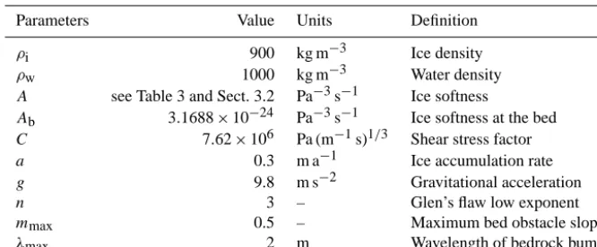
Table 2. Parameter values used for all experiments.
Parameters Value Units Definition
ρi 900 kg m−3 Ice density
ρw 1000 kg m−3 Water density
A see Table 3 and Sect. 3.2 Pa−3s−1 Ice softness
Ab 3.1688×10⁻²⁴ Pa−3s−1 Ice softness at the bed
C 7.62×10⁶ Pa (m−1s)1/3 Shear stress factor
a 0.3 m a−1 Ice accumulation rate
g 9.8 m s−2 Gravitational acceleration
n 3 – Glen’s flaw low exponent
mmax 0.5 – Maximum bed obstacle slope
λmax 2 m Wavelength of bedrock bumps
At the grounding line, the requirement of exact flotation leads to the boundary condition
H=ρw
ρib at x=xg. (9) Combining Eqs. (2)–(5), the stress balance in the ice shelf is given by
h
2A¯−1nH|ux|
1
n−1ux i
x −ρi
1− ρi
ρw
gH Hx=0. (10)
At the calving front the ice shelf is subject to the ocean back pressure, pw= −ρwgz, between the ice shelf base, z=(ρi/ρw)H, and sea level, z=0. The ocean pressure partially (but not com-pletely) balances the hydrostatic pressure of the ice, pi= −ρig(z−s). The force on the ice shelf due to the difference in hydrostatic pressure between the ice shelf and the ocean is
fp(xc)=
s Z
−(ρi/ρw)H
−ρig(z−s)dz− 0
Z
−(ρi/ρw)H
−ρwgzdz
=1
2ρi
1− ρi
ρw
gH2. (11)
The force on the calving face due to longitudinal (viscous) stress must compensate for this imbalance in hydrostatic pressure:
2A¯−1nH|ux|
1
n−1ux=1
2ρi
1− ρi
ρw
gH2 atx=xc. (12) Following Schoof (2007a), we integrate Eq. (10) from the calving front (x=xc) to the grounding line (x=xg), and use Eq. (12) to show that the same condition holds at the ground-ing line as at the calvground-ing front:
2A¯−1n
H|ux|
1
n−1ux=1
2ρi
1− ρi
ρw
gH2 atx=xg. (13) In order for the stresses to remain finite,H,uandux must
be continuous across the grounding line.
2.2 Effective pressure parameterization and friction law
Most models of marine ice sheets assume that the basal fric-tion jumps discontinuously to zero across the grounding line. We propose a simple parameterization that removes the dis-continuity, yielding a smooth transition between grounded and floating ice. We adopt the friction law from Schoof (2005), validated and extended in Gagliardini et al. (2007). This formulation, given by Eq. (6), has the correct limits for large values of the effective basal pressureN and slow flow, and reduces to Coulomb friction in the limit of smallN and fast flow. Schoof (2005) suggested that this friction law is an appropriate simplification for rough terrain; Gagliardini et al. (2007) showed that this limiting case of their more general friction law (corresponding to their decay parameterq=1) was appropriate for sawtooth terrain. They also argued that this limit of their friction law may lead to better behavior in numerical models because the relation between basal stress and sliding velocity is monotonic.
If the effective pressure is continuous across the grounding line, the basal shear stress smoothly approaches zero at the grounding line. Assuming that the subglacial drainage sys-tem is connected to the ocean, the water pressure at the ice-sheet base will be close to the ocean pressure at that depth, reaching the ocean pressure at the grounding line (with pres-sure differences driving flow through the drainage system). A simple function for the effective pressure that accounts for connectivity between the subglacial drainage system and the ocean is
N (p)=ρigH
1−Hf
H
p
, (14)
in which we introduce a parameterpthat varies between zero (no basal water pressure) and one (the subglacial drainage system is hydrologically well connected to the ocean). The flotation thickness is defined byHf≡max0,ρw
ρib
– When p=0, N (p)=ρigH (no water-pressure sup-port).
– Whenp=1,N (p)=ρig (H−Hf)(full water-pressure support from the ocean wherever the ice-sheet base is below sea level).
– At the grounding line whenp >0,N (p)=0 (τbis con-tinuous across the grounding line).
– Far from the grounding line (where the bed is above sea level andHf=0),N (p)=ρigH.
WhenHf/H1 and the bedrock is below sea level (b >0), the basal water pressure is attenuated to a fractionpof the full ocean pressure at the depth of the bed (see Appendix A). These conditions will typically hold on the inland side of the transition zone, since a rapid increase inHis usually needed to produce the driving stress that balances the relatively large basal friction in this region. One way such attenuation might occur is by a gradual loss of connectivity between the basal hydrological system and the ocean.
Equation (14) can be regarded as a mathematical regular-ization, ensuring that the basal friction transitions smoothly from a finite value in the ice sheet interior to zero in the ice shelf. It can also be viewed as a simple parameterization of basal hydrology, motivated by the hydrological connectiv-ity that may exist between the ice bed and the ocean near the grounding line. (By “parameterization” we mean the re-placement of small-scale or complex physical processes with a simplified process.) The functional form of Eq. (14) is ad hoc, since there are no detailed observations to show how N varies near grounding lines, but the limits are physically based.
We emphasize that Eq. (14) does not represent all the pro-cesses that might be included in a complex hydrology or till model. It represents only the portion of water-pressure sup-port related to the ocean; basal water pressure in the model falls to zero when the bedrock reaches sea level (b=0). More sophisticated models of basal till find that the basal wa-ter pressure remains a significant fraction of the overburden pressure in much of the ice-sheet interior (Tulaczyk et al., 2000b; van der Wel et al., 2013). A more complex model might include a network of channels as well as water-laden till at the base of ice streams. This hydrological network would influence the basal friction through water-pressure support outside the transition zone. Thus, our parameteriza-tion predicts a larger N away from the grounding line than would likely be observed in much of the interior of ice sheets. We do not think this is a critical model weakness, however, because we are mainly interested in ice dynamics near the grounding line. In the interior, whereN is larger, the basal shear stress is described by a power law (see Eq. (16) below) and is relatively insensitive toN.
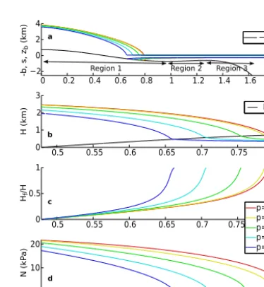
Figures 1 and 2 show typical ice-sheet geometry, thick-ness,Hf/H andN for five values ofpover linear and poly-nomial bedrock topography, respectively. In both cases, the
Ice sheet domain (103km)
N (
kP
a)
Hf
/H
H (
km)
-b,
s
,
zb
(
km)
0 0.2 0.4 0.6 0.8 1 1.2 1.4 1.6 1.8 2 −2
0 2 4
0.7 0.8 0.9 1 1.1 1.2
0 2 4
Hf
0.7 0.8 0.9 1 1.1 1.2
0 0.5 1
0.7 0.8 0.9 1 1.1 1.2
0 10 20 30
p=0 p=0.25 p=0.5 p=0.75 p=1
−b
a
b
c
d
Figure 1. Dependence of ice geometry and effective pressure on
the parameterp over a linear bed as in Schoof (2007b). All pan-els show the fixed-grid solution at 0.8 km resolution without a grounding-line parameterization (see Sec. 2.3) and with ice soft-nessA=10−25Pa−3s−1. (a) Ice surface and bedrock (colors), and basal elevation (black) over the full ice-sheet domain. (b) Ice sheet thickness (colors) and flotation thickness (black) over the marine portion of the ice sheet. (c) The ratio between the flotation thickness and the ice-sheet thickness. (d) The effective pressureN, which ap-proaches zero more smoothly with increasingp. Plots in panels (c) and (d) include only grounded cells, as the ice is exactly at flotation and effective pressure is zero elsewhere. The plotted effective pres-sure does not go to zero for allp >0 because the grounding line lies between the last grounded cell and the first floating cell.
Ice sheet domain (103 km)
N (
kP
a)
Hf
/H
H (
km)
-b,
s
,
zb
(
km)
0 0.2 0.4 0.6 0.8 1 1.2 1.4 1.6 1.8 −2
0 2 4
−b
0.5 0.55 0.6 0.65 0.7 0.75 0.8 0
1 2 3
Hf
0.5 0.55 0.6 0.65 0.7 0.75 0.8 0
0.5 1
0.5 0.55 0.6 0.65 0.7 0.75 0
10 20
p=0 p=0.25 p=0.5 p=0.75 p=1 Region 1 Region 2 Region 3
d c b a
smaller thepvalue the greater the effective pressure, which tends to move the grounding line seaward. The jump in ef-fective pressure is to be expected for p=0 because of the limit defined above. For small values of p >0, the transi-tion in basal stress occurs over a narrow region of order 1 km or less, and is thus resolved only at high model resolution. The figures show thatN drops to zero more smoothly asp increases, meaning that the basal stress will also be increas-ingly smooth.
Parameterized in terms ofp, Eq. (6) becomes
τb=C|u|
1
n−1u
N (p)n
κ|u| +N (p)n n1
, (15)
whereκ≡ mmax
λmaxAb. This formulation does not require the
in-troduction of an arbitrary length scale of basal transition, as in the parameterization proposed by Pattyn et al. (2006). Equation (15) has two asymptotic behaviors. In the ice sheet interior, the ice is thick and slow-moving, so that κ|u|
N (p)nand τb≈C|u|
1
n−1u. (16)
In this limit,τbis independent ofp. Many models define the basal-friction law throughout the ice sheet to have the form of Eq. (16), as in Schoof (2007a) and the MISMIP exper-iments. This simplified friction law leads to a set of equa-tions with an accurate semi-analytic approximation (Schoof, 2007a, b), whereas the more complex friction law in Eq. (15) does not lend itself to a similar semi-analytic solution (see Appendix B). A boundary-layer solution could be computed numerically, but we have instead opted to compute a high-accuracy benchmark solution over the full domain, as de-scribed in the next section. The semi-analytic solution of Schoof (2007a) closely approximates our model as p ap-proaches zero. Figure 3a shows that the basal-stress term (blue) closely matches the limit of high overburden pres-sure (red) given by Eq. (16) when p=0. In this limit, the boundary-layer solution and our high-resolution benchmark solution differ by a few kilometers or less.
The second asymptote, the Coulomb-friction limit, occurs near the grounding line where the ice is thin and fast-flowing, so thatκ|u| N (p)nand
τb≈ C
κ1n
N (p) u
|u|. (17)
By construction, whenp=0 the effective pressure is equal to the full overburden pressure,pi, and the basal stress dis-continuously drops to zero across the grounding line. When p >0, the effective pressure N smoothly approaches zero at the grounding line over a distance that increases asp in-creases. Just inland of the grounding line, the basal stress is proportional to the effective pressure.
We define the friction transition zone as the part of the ice sheet where 0≤N (p)n< κ|u|, where Coulomb friction
is dominant. The friction transition zone is closely related to the transition zone defined in Sect. 1, since the transition from flow dominated by vertical shear to flow dominated by extensional stress must occur in the region where the basal shear stress drops from a large value (highN) to a small value (lowN). For the range of parameters we studied, the size of the friction transition zone varies between 0 and∼20 km, depending onp, the bedrock topography, and the ice soft-ness. Importantly, the size of the friction transition zone is an increasing function ofp, meaning that, at a given resolu-tion, this zone is better resolved whenpis larger. Figure 3b and 3c show the basal-stress terms and their two asymptotic limits forp=0.5 andp=1, respectively. Eq. (16), the red curve, dominates in the bulk of the ice sheet, while Eq. (17), shown in green, dominates in the friction transition zone.
The size of the friction transition zone depends on κ≡ mmax
λmaxAb as well as p. For this study we chose the values of
mmax,λmax, andAbas in Pimentel et al. (2010) and given in Table 2. Since the focus of this paper is on the effect of our effective-pressure parameterization near the grounding line, we defer to a follow-up study a full analysis of how variation ofκaffects our results at different values ofpandA. Here we simply summarize what we observed for a specific ice soft-nessA=4.6416×10⁻²⁵Pa−3s−1. Increasingκby an order of magnitude introduces a finite friction transition zone of
∼1 km whenp=0 and triples the size of the friction tran-sition zone to∼ 28 km when p=1. Although the friction transition zone becomes finite whenp=0, the basal fric-tion remains discontinuous across the grounding line. Even so, a larger value ofκ could decrease the model resolution required for small values ofp. Decreasingκ by an order of magnitude has no impact on the friction transition zone when p=0, but halves the friction transition zone to∼5 km when p=1. More generally, asκ goes to zero the basal friction law will asymptote to Eq. (16), regardless ofp.
Figures 1–3 show that although the friction transition zone is small compared to the whole ice sheet, its effects are far-reaching. As p increases from 0 to 1 (other things being equal), the grounding line retreats by more than 100 km, and the steady-state surface elevation is reduced hundreds of km upstream.
2.3 Numerics
Basal stress term (kPa)
Distance to grounding line (km)
a) p = 0 b) p=0.5 c) p=1
40 20 0
0 50 100 150 200 250
40 20 0
0 50 100 150 200 250
40 20 0
0 50 100 150 200 250
Figure 3. Basal stress given by Eq. (15) (blue) and its
asymp-totic limits, Eq. (16) (red) and Eq. (17) (green) for ice softness
A=10−25Pa−3s−1and using the Chebyshev benchmark solution.
(a) Whenp=0, the second (green) asymptote is never reached, the red and blue curves overlap almost exactly, and there is no friction transition zone (basal stress falls abruptly to zero at the grounding line). (b) and (c) Whenp=0.5 andp=1, the length of the fric-tion transifric-tion zone, defined as the region where 0≤N (p)n≤κ|u|
(roughly speaking, the region where the blue curve differs from the red curve), ranges from several hundred meters to 20 km depending onA,pand bedrock topography.
computational cost. As we will show in Sect. 3, depending on the values of the parameterp, our parameterization of ef-fective pressure can considerably reduce the computational cost of an accurate fixed-grid simulation.
Pattyn et al. (2006) and Gladstone et al. (2010a) showed that numerical errors (or alternatively, the computational cost of a simulation with a given numerical error) could be re-duced through the use of numerical grounding-line param-eterizations (GLPs). GLPs involve sub-grid-scale interpola-tion of the grounding-line posiinterpola-tion, which is used in the grid cell containing the grounding line to compute a stress that varies continuously as the grounding line moves.
In the following section, we present results both with and without a GLP in order to compare our findings with those of Gladstone et al. (2010a) and to investigate the possible bene-fit of combining the GLP with our effective-pressure param-eterization. We implemented a GLP similar to the PA_GB1 GLP in Gladstone et al. (2010a). First, we determine the grounding-line position based on linear interpolation of the functionf≡Hf/H, given thatf =1 at the grounding line. Then, in the cell containing the grounding line, we compute the basal and driving stresses once each assuming that the cell is entirely grounded and then entirely floating. Finally, the stresses are linearly interpolated between their grounded and floating values, based on the fraction of the cell that is grounded vs. floating. The resulting expressions for the basal and driving stresses are given by Eqs. (C38) and (C39) re-spectively. We chose not to use the quadrature methods
em-H1 H2
u3/2
HN
uN+1/2
x=0 x=xc
Δx
HN+M
uN+M+1/2
Ice Sheet Ice shelf
Figure 4. Illustration of the staggered grid used in the model. The H-grid points are represented by solid circles and theu-grid points by empty circles.1xis the grid spacing (on bothH- andu-grids).
HNis the ice thickness in the last grounded point. The ice divide is
atx=0 and the calving front atx=xc.
ployed in Gladstone et al. (2010a) because they would likely be too cumbersome and costly in 3-D ice-sheet models. In simulations without a GLP, the model computes basal and driving stresses as if the cell containing the grounding line were entirely grounded.
We discretize the equations of motion on a staggered grid, shown in Fig. 4, with alternating velocity and thickness points (u- andH-points). The ice divide (x=0) and the calv-ing front are placed at au-point and anH-point, respectively, allowing us to satisfy both boundary conditions naturally. We included a ghostH-point to the left of the ice divide to ensure zero surface slope at the divide. The details of the numerics for the fixed-grid model are given in Appendix C1, and a full description of the GLP is given in Appendix C2.
To evaluate the performance of the fixed-grid model, we needed a benchmark solution to compare with our fixed-grid results. To this end we implemented a stretched-grid, pseudo-spectral method using Chebyshev polynomials (Boyd, 2001) to produce spectrally accurate steady-state benchmark re-sults. The Chebyshev collocation points are non-uniformly distributed over the ice-sheet domain, with the highest res-olution at the grounding line and ice divide. Using 1025 Chebyshev modes, the grid spacing continuously decreases from∼80 m at a distance of 2 km from the grounding line to∼2.5 m at the grounding line. We verified the numeri-cal convergence of the Chebyshev benchmark by compar-ing groundcompar-ing-line positions with those computed uscompar-ing 2049 modes at various values ofp andA. We found that results changed by at most 50 cm when doubling the resolution, sug-gesting that numerical errors in the Chebyshev grounding-line position are negligible compared to those from the fixed-grid model.
stresses, use the friction law from Eq. (16), and apply bound-ary conditions given by Eqs. (9) and (13). (This approach can be used to reproduce the grounding-line position from Model A but not the velocity and thickness solutions.)
When we included the full longitudinal stress in the Chebyshev model, the differences with the Model A grounding-line position increased to ∼1 km. Switching to the more complex basal friction law, Eqs. (14) and (15), in-troduced further differences of∼1 km or less. We attribute the differences between Model A and the Chebyshev solu-tion with full longitudinal stress and our fricsolu-tion law to the simplifying assumptions of Model A, rather than to errors in the Chebyshev model. These results give us confidence that the Chebyshev model is producing solutions with errors that should be negligible (of order meters or less) compared to those from the fixed-grid model (order kilometers or more).
This close agreement between the boundary-layer model and our benchmark sheds some light on possible sources of discrepancies between numerical solutions in Pattyn et al. (2012). While some discrepancies are due to numerical er-ror, others are due to different model formulations. The lat-ter is evident in Durand et al. (2009). Whereas they found poor agreement between their Stokes-flow model and the boundary-layer Model B from Schoof (2007a) – which might reflect the differences between a Stokes model and a depth-integrated model – we find excellent agreement between our benchmark (withp=0) and the boundary-layer model, both of which aim to solve the same equations.
The full details of the method are given in Appendix C3.
3 Results
The results described in this section are based on the MIS-MIP experiments (Pattyn et al., 2012), which are designed to study the transient behavior of marine ice-sheet models. For a given ice softnessAwe obtain a steady ice-sheet pro-file. This profile is then used as the initial condition for the next experiment, which evolves to a new steady state with a new value of the ice softness. MISMIP experiment 1 pre-scribes decreasing values ofAand linear bedrock topogra-phy, leading to an advancing grounding line. MISMIP ex-periment 2 is exex-periment 1 in reverse, whereAis increased back to its original value, resulting in grounding-line re-treat. Experiment 3 is similar to the combination of exper-iments 1 and 2, but using a polynomial bedrock topography. A full description of the MISMIP experiments can be found at http://homepages.ulb.ac.be/~fpattyn/mismip/.
Models participating in the MISMIP intercomparison used the friction law of Schoof (2007a), which is equivalent to Eq. (16). For our experiments we test two model configu-rations, non-GLP and GLP, both of which include the fric-tion law from Eq. (15), with effective pressure defined by Eq. (14). The GLP configuration includes the grounding-line parameterization discussed in Sect. 2.3 and Appendix C2,
while the non-GLP configuration does not. We tested five values of the parameterp, equally spaced between zero and one, at seven resolutions between 3.2 and 0.05 km, each a factor of two smaller than the previous. Only the results with p=0 can be directly compared with the results of Pattyn et al. (2012). By changing p we are changing the physics, not just the numerics, of the problem. Aside from the modi-fied friction law and associated parameterization of effective pressure, we used the standard MISMIP protocols except as specifically stated below.
Typically, differences in grounding-line positions are used to compare the accuracy of ice-sheet model results (Pattyn et al., 2012). This error metric is practical for us as well, since the grounding-line position is easily diagnosed from both Chebyshev and fixed-grid simulations. In realistic simu-lations, errors in grounding-line position are not as important as those in volume above flotation, which is directly related to the ice sheet’s contribution to sea-level change. However, we found (not shown) that the behavior of both metrics is qualitatively similar: larger errors in grounding-line position correspond to larger errors in volume above flotation. 3.1 Linear-bed experiments
We performed a series of experiments with the linear bedrock topography of Schoof (2007a), shown in Fig. 1a:
b(x)= −720−778.5 x 750 km
m. (18)
We forced the ice sheet first to advance and then to retreat by varying the ice softness A, in analogy to MISMIP ex-periments 1 and 2 (Pattyn et al., 2012). To force ice-sheet advance, we incrementally decreasedAthrough the values listed in Table 3, allowing the ice sheet to evolve to steady state each timeA was changed. Then, to force retreat, we increasedAthrough the same values in reverse order, again evolving to steady state at each step. Experiments were per-formed at seven resolutions (3.2, 1.6, 0.8, 0.4, 0.2, 0.1 and 0.05 km), five values ofp(0, 0.25, 0.5, 0.75 and 1), and both with and without the GLP.
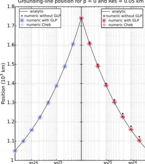
Schoof (2007a, b) showed that the steady-state grounding-line position on a bed sloping monotonically downward in the direction of the ice flow is unique for a given ice soft-ness. Figure 5 shows the grounding-line positions derived from the boundary-layer solution of Schoof (2007a) and those from advance-and-retreat cycles using our Chebyshev and fixed-grid models withp=0 at 0.05 km resolution. The grounding-line position in our Chebyshev simulation differs from that of the boundary-layer solution by less than 1.2 km. As mentioned in the previous section, this difference appears to be mostly due to the fact that the boundary-layer model neglects longitudinal stresses in the bulk of the ice sheet.
Grounding-line position for p = 0 and Res = 0.05 km
Positio
n
(1
0
3 k
m
)
1/A
1024 1025
1 1.1 1.2 1.3 1.4 1.5 1.6 1.7 1.8
analytic numeric without GLP
numeric with GLP numeric Cheb
1024
1025 analytic numeric without GLP
numeric with GLP numeric Cheb
Figure 5. The grounding-line position during advance and retreat
experiments over a linear bed at 50 m resolution withp=0 from the boundary-layer solution by Schoof (2007a) (solid black), the Chebyshev benchmark model (pluses), the fixed-grid model with-out the GLP (dots) and the fixed-grid model with the GLP (stars). The boundary-layer solution is in close agreement with the Cheby-shev benchmark (maximum difference of 1.2 km), as are the fixed-grid results with or without the GLP. Both fixed-fixed-grid models closely agree with the Chebyshev benchmark during advance (maximum difference of 1.2 km). During retreat, the model with the GLP matches the benchmark (maximum difference of 5 km) better than the model without the GLP (maximum error of 26 km).
experiment, the grounding-line position is overestimated as much as 26 km when the GLP is not used, but by no more than 5 km with the GLP included, thereby showing its poten-tial benefit.
Figure 6 shows the differences between the grounding-line position from the fixed-grid and benchmark models in several configurations: both without (left) and with (right) the GLP, and at three different resolutions, 1.6 km (top), 0.4 km (mid-dle) and 0.1 km (bottom). We show differences rather than es-timated errors (the absolute value of the differences), because the sign of the difference is important in telling whether the grounding line is too far advanced or too far retreated. Dur-ing the retreat phase of each experiment (the right-hand side of each plot), the fixed-grid grounding line is always too ad-vanced, whereas during the advance phase (the left-hand side of each plot), the grounding line may be too advanced or too retreated depending on the values of p andA. For simula-tions withp <0.5 with and without the GLP, the
grounding-Table 3. Values of the ice softnessAused in the MISMIP experi-ment 1 (linear bed). These are the same values prescribed in Pattyn et al. (2012).
Step no. A(×10−26s−1Pa−3)
1 464.16
2 215.44
3 100
4 46.416
5 21.544
6 10
7 4.6416
8 2.1544
9 1
Re
s
= 0
.1
k
m
Re
s
= 0
.4
k
m
Re
s
= 1
.6
k
m
1/A 1/A
Without GLP With GLP Difference in grounding line position
Di
ff
er
en
ce
(k
m
)
50 30 100 10 30 50 250 500
50 30 100 10 30 50 250 500
50 30 100 10 30 50 250 500
50 30 100 10 30 50 250 500
102410251026 50
30 100 10 30 50 250 500
1024
1025 50 102410251026 30
100 10 30 50 250 500
1024 1025 p=0
p=0.25 p=0.5 p=0.75 p=1
-Figure 6. The signed difference between the fixed-grid and
bench-mark grounding-line positions over a linear bed at 1.6 km (top row), 0.4 km (middle row) and 0.1 km (bottom row) resolution for sim-ulations without GLP (left column) and with GLP (right column). Each column contains both advance (left of each panel) and retreat (right of each panel) experiments. The dashed line (at 50 km) in each panel shows the location of a transition in scale of they-axis, which allows the same figure to present both very large and rel-atively small errors. Errors (the magnitude of the differences) are approximately inversely proportional to the resolution and decrease with increasingp, strongly so without the GLP. The GLP reduces the most egregious errors during retreat (occurring whenpis small).
Without GLP With GLP Maximum Error in grounding line position
R
esol
u
ti
on
(
km
)
p p
0 0.25 0.5 0.75 1
3.2
1.6
0.8
0.4
0.2
0.1
0.05
1 10 30 80 200 400 680
0 0.25 0.5 0.75 1
3.2
1.6
0.8
0.4
0.2
0.1
0.05 0
1 10 30 75 125
0
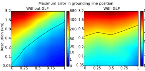
Figure 7. The maximum error over the advance and retreat
exper-iments between the fixed-grid and benchmark grounding-line posi-tion over a linear bed for simulaposi-tion without the GLP (left column) and with the GLP (right column). The errors are bilinear interpola-tions of our 35 experiments (5 values ofpand 7 resolutions). The black line shows a contour of 30 km error (∼5 % of the differ-ence between the most advanced and the most retreated positions of the benchmark), below which we deem the error to be suffi-ciently small. Note that each panel uses a different nonlinear color bar. Without the GLP, the maximum error decreases approximately linearly with resolution and superlinearly withp. With the GLP the maximum error decreases weakly with respect top but approxi-mately linearly with resolution.
Figure 7 shows the maximum error over an advance-and-retreat cycle at a given value of p and resolution without the GLP (left) and with the GLP (right). The error map was obtained by bilinear interpolation from our 35 experi-ments. The figure shows that the maximum errors decrease approximately linearly with the grid-cell size for each value ofp, either with or without the GLP. Linear convergence of grounding-line errors with resolution has been seen in other fixed-grid models (Gladstone et al., 2010a; Cornford et al., 2013). Compared with resolution, the application of the GLP and larger values of the parameterp produce a much more dramatic reduction in maximum error.
The differences between experiments are most apparent during the retreat phase of each experiment (right-hand side of each panel in Fig. 6). The experiments most similar to typ-ical MISMIP fixed-grid results – experiments without GLP and withp=0 – show huge estimated errors during retreat on the order of hundreds of kilometers. The maximum er-ror is approximately a factor of ten smaller in both the ex-periments with a GLP at p=0 (red dots in the right-hand column) and the experiments without a GLP but with p=
1. Surprisingly, the combination of the GLP and effective-pressure parameterization withp=1 does not seem to pro-duce smaller errors thanp=1 without the GLP, showing di-minished performance particularly during retreat. The GLP has essentially no impact on the advance phase (left-hand side of each panel in Fig. 6), whereas the error during ad-vance does tend to decrease aspincreases.
The black line in Fig. 7 shows a maximum error in grounding-line position of∼30 km (∼5 % of the difference
between the most advanced and most retreated grounding-line positions of the benchmark). We chose this as a (some-what arbitrary) threshold below which we deem the error to be acceptable. In experiments without the GLP, smoother basal friction (larger values ofp) means that this error thresh-old has reached a coarser resolution. This is not the case when the GLP is included. Instead we reach our threshold error at roughly the same resolution for all values ofp. As it turns out, using the GLP is always beneficial whenp≤0.5 but becomes disadvantageous whenp >0.5.
3.2 Polynomial-bed experiments
We performed a second series of grounding-line advance-and-retreat cycles with bedrock topography shown in Fig. 2a and given by the following polynomial function (Schoof, 2007a):
b(x)= −
729−2184.8 x 750 km
2
+1031.72 x 750 km
4
−151.72 x 750 km
6
m. (19)
These experiments are analogous to MISMIP experiment 3 (Pattyn et al., 2012), but with our modified friction law and effective-pressure parameterization and with more values of the ice softness A. The bed topography has three distinct regions. Region 1 slopes downward from the ice divide to-ward a local minimum, region 2 slopes upto-ward, and region 3 slopes downward again, forming a steep continental-shelf break.
Theoretical arguments (Weertman, 1974; Schoof, 2007a) suggest that stable steady-state grounding-line positions can be found in regions 1 and 3 (with downward-sloping beds) but not in region 2 (with an upward-sloping bed). Our numer-ical results are consistent with theory. We found that steady-state grounding-line positions do not exist on upward-sloping beds in region 2 but that new steady state solutions are found in region 3 when the grounding line has been forced to ad-vance through region 2.
Grounding-line position for p = 0 and Res = 0.05 km
Positio
n
(1
0
3 k
m
)
1/A 1025
0.7 0.8 0.9 1 1.1 1.2 1.3 1.4
1025 analytic
numeric without GLP numeric with GLP numeric Cheb
analytic numeric without GLP
numeric with GLP numeric Cheb
Figure 8. As in Fig. 5 but with the polynomial bed shown in Fig. 2a.
The boundary-layer solution closely agrees with Chebyshev results (maximum difference of 1.4 km). Fixed-grid results both with and without the GLP closely agree with the Chebyshev benchmark dur-ing advance (maximum difference of∼1 km without the GLP and
∼1.6 km with the GLP). During retreat, the model with GLP is the better match to the benchmark (maximum difference of∼14 km). Without the GLP, the fixed-grid grounding-line position matches the benchmark reasonably well when both solutions are on the same side of the unstable region (maximum difference of∼38 km) but not in the vicinity of the local maximum where the solutions are on different side of the unstable region, (maximum difference of
∼570 km).
range ofAto 2.5×10⁻²⁷s−1Pa−3and variedAover 34 val-ues approximately equally spaced in log space. For all exper-iments, we used more values ofAthan MISMIP in order to obtain a better statistical sampling of the error within each experiment and to reduce the influence of particularly large errors that occur as the grounding line approaches the un-stable region. The largest errors occur when the fixed-grid solution is in region 1 while the benchmark is in region 3 or vice versa.
When p=0, the boundary-layer solution, model A of Schoof (2007a), again provides a good approximation of our equations of motion. Figure 8 shows the grounding-line positions derived from the boundary-layer solution together with the positions from experiments using our Chebyshev and fixed-grid models withp=0. The grounding line of the boundary-layer solution differs from that in our Chebyshev benchmark simulations by less than 1.4 km, similar to the linear bed experiments. The fixed-grid model at 0.05 km res-olution performs well during the advance phase both with
Without GLP With GLP
RMS Error in grounding line position
0 0.25 0.5 0.75 1
3.2
1.6
0.8
0.4
0.2
0.1
0.05 0
30 90 150 210 270 330
0 0.25 0.5 0.75 1
3.2
1.6
0.8
0.4
0.2
0.1
0.05
R
esol
u
ti
on
(
km
)
p p
Figure 9. The root-mean-square (RMS) error between the
fixed-grid and benchmark grounding-line position over a polynomial bed for simulation without the GLP (left column) and with the GLP (right column). The errors are bilinear interpolations of our 35 experiments. The gray area shows experiments that were not re-versible (i.e., for which the fixed-grid grounding line position did not retreat from region 3 to region 1 during the retreat experiment). The black line shows a contour of 30 km error, below which the error is deemed acceptable, as in Fig. 7. The RMS error without the GLP is approximately inversely proportional to the resolution and decreases strongly with increasingp. With the GLP, the RMS error is inversely proportional to the resolution and decreases, though less steeply, with increasingp.
and without the GLP; the grounding line is always in the same region (either 1 or 3) as the benchmark solution. The maximum error is about 0.9 km without the GLP and about 1.6 km with the GLP. However, without the GLP, the model does not perform as well during the retreat phase. The error in the grid solution is as large as 38 km when the fixed-grid and benchmark grounding lines are in the same region. The fixed-grid model with the GLP follows the Chebyshev solution more accurately, with a maximum error of∼14 km and grounding-line positions that always lie in the same re-gion as the benchmark.
During the retreat experiment, the model configuration without GLP shows a grounding-line position located in the wrong region for two values of A, leading to an error of about 570 km. Although this behavior is not seen when the GLP is included, we would likely see similar discrepancies between this configuration and the benchmark if we had sampled an even larger number of Avalues. In other words, the GLP would appear to reduce the likelihood of these large errors but it is unlikely that they have been eliminated entirely.
interpolation from our 35 experiments. Here, we used the RMS error instead of the maximum error because the lat-ter is typically dominated by cases in which the benchmark and fixed-grid grounding lines lie in different regions and is highly sensitive to the particular choice ofAvalues. The gray area in each panel indicates experiments which are not re-versible (the fixed-grid grounding line position fails to retreat back to region 1 at the end of the retreat experiment). The figure shows that, without the GLP, the RMS error decreases linearly with resolution and rapidly with increasingp. When the GLP is included, the RMS error decreases linearly with resolution, while increasingphas a less dramatic impact. As was the case for the linear bed experiments, including the GLP improves the error for small values but not necessarily for large values of p. For smallp, including the GLP im-proves the ability of the model to retreat past the unstable region, as shown by the reduced grey area on the right-hand side of Fig. 9. All experiments with the GLP and a resolution of ∼1 km or higher show reversibility, whereas a resolution of between 100 and 200 m is required without GLP when p=0.
Similarly to the previous section, we use a threshold of 30 km as the maximum allowable RMS error, indicated by the black contour line in Fig. 9. Our results show that even with the GLP, resolution as high as 100 m is required in lo-cations with large effective pressure near the grounding line (p∼0). On the other hand, a resolution of∼1 km is suffi-cient where the effective pressure is low (p∼1). In general, the results from the linear section remain valid when using a polynomial bed: When p≤0.5, using the GLP leads to smaller RMS errors and better reversibility. However, when p >0.5, using a GLP is disadvantageous.
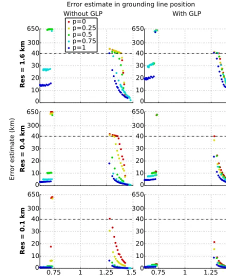
Figure 10 shows the error in grounding-line position as a function of the benchmark grounding-line position during the retreat phase. The figure makes clear that the error in-creases as the grounding line approaches the unstable re-gion. These results suggest that the fixed-grid model can cap-ture hysteresis with increasing fidelity aspincreases and (to a lesser extent) as resolution increases, and that errors nearly always decrease at a given value ofxgaspincreases.
Figure 10 also suggests that errors may be a strong func-tion of bedrock slope. The largest errors occur near the local maximum in bed elevation at aroundx=1.25×10³km, and decrease sharply as the bedrock steepens further into region 3. This behavior is to be expected as the grounding line ap-proaches a bifurcation point. No stable steady-state solution will exist near that maximum ifAis decreased further; small changes in A will lead to large changes in grounding-line position. Similar inverse correlation between bed slope and error can be seen in region 1, though the bedrock steepens more gradually in this region.
Re
s
= 0
.1
k
m
Re
s
= 0
.4
k
m
Re
s
= 1
.6
k
m
GL position (103 km) GL position (103 km)
Without GLP With GLP Error estimate in grounding line position
E
rr
o
r
est
im
at
e (
km)
0 10 20 30 40
0 10 20 30 40 300 650
0 10 20 30 40
0 10 20 30 40 300 650
0.75 1 1.25 1.5 0
10 20 30 40
0.75 1 1.25 1.5 0
10 20 30 40 300 650 p=0
p=0.25 p=0.5 p=0.75 p=1
300 650 300 650 300 650
Figure 10. As in Fig. 6, but showing only the retreat experiment
over the polynomial bed and with benchmark grounding-line po-sition instead ofAalong thex-axis. The dashed line (at 40 km) in each panel shows the location of a transition in scale of they -axis used to show large errors without losing the differences be-tween smaller errors. The error in grounding-line position is consis-tently lower at a given grounding-line position whenp=1 than for smaller values ofp. The figure shows that errors tend to increase as the grounding line approaches the unstable region (empty gap in each figure).
4 Discussion
Previous studies of marine ice-sheet dynamics have sug-gested that grounding-line position converges with increas-ing resolution (Vieli and Payne, 2005), typically linearly (Gladstone et al., 2010a; Cornford et al., 2013). We find this to be true in our simulations. However, we do not observe the numerical instability seen at coarser resolution in Gladstone et al. (2010a) or the premature retreat found in the fixed-grid model of Goldberg et al. (2009), as seen in their Fig. 4b. In-stead, with the use of our basal-friction parameterization and assuming good connectivity to the ocean (p∼1), we find that a fixed-grid model can yield accurate results at relatively coarse resolution. These improvements do not require mod-ified numerical techniques, such as a GLP, but arise from plausible changes in model physics.
or coarser when the basal shear stress smoothly approaches zero near the grounding line. Much finer resolution,∼500 m in the linear bed experiment and∼100 m in the polynomial bed experiment, is required when the basal stress is discon-tinuous at the grounding line. More realistic models using discontinuous basal stress have shown accurate grounding-line migration only with a resolution of 200 m or less (Corn-ford et al., 2013), consistent with our simulations. Our results suggest that it may be possible to simulate marine ice sheets at much lower computational expense than would be required with traditional friction laws. Models with adaptive and un-structured grids (Goldberg et al., 2009; Favier et al., 2012; Perego et al., 2012; Cornford et al., 2013) could be made more computationally efficient by reducing the need for very fine resolution near grounding lines. Also, our parameteriza-tion might allow uniform-grid models to simulate whole ice sheets, since ∼1 km resolution throughout the ice sheet is feasible (though expensive). However, this could require set-tingp∼1 everywhere in the ice sheet, which might not be physically realistic for some regions.
Our one-dimensional model has several simplifying as-sumptions that may limit its applicability to real ice sheets. Notably, the model does not include vertical shear stress (so it cannot simulate flow over a frozen bed) or lateral shear stress (so it does not include effects of ice-shelf buttressing). These missing stresses are likely to be large enough (Whillans and van der Veen, 1997; Schoof, 2007a) that we cannot validate our results by direct comparison to observations. In particu-lar, Goldberg et al. (2009) showed, in a series of experiments with basal stress corresponding to ours whenp=0, that but-tressing can affect the rate and direction of grounding-line advance or retreat over upward-sloping beds. Gladstone et al. (2012) showed that buttressing can relax the requirement for high resolution, so that without buttressing, a model always requires higher resolution than if buttressing is included. This may imply that our results can be considered an upper bound in model resolution requirement.
Most large-scale ice-sheet models do not explicitly model basal hydrology, but instead use inversion to compute a spa-tially variable basal sliding coefficient based on observations. (The basal sliding coefficient is typically equivalent to C in Eq. 16). In some cases the basal sliding coefficient ob-tained by inversion decreases to zero at or near the ground-ing line (Vieli and Payne, 2003; Larour et al., 2012), sug-gesting that (in the terms of our model) p >0. In ice-sheet models that invert for a spatially varying parameterC(or its equivalent), the inversion process will tend to find a value of C that is close to zero near the grounding line in re-gions with significant basal-water support, leading to an ini-tial τb that is continuous (or nearly continuous) across the grounding-line. However, in the absence of a basal-friction law that responds to changes in the grounding-line location, the grounding line will migrate over time butC will remain fixed in space. This is likely to lead to large jumps in basal stress across the grounding line at later times, and to
non-convergent grounding-line dynamics at coarser resolution. An advantage of our parameterization is that, for larger val-ues ofp, the basal stress remains continuous and smooth over a resolvable friction transition zone even as the grounding line moves.
We plan to incorporate our parameterization in the Com-munity Ice Sheet Model (CISM), a three-dimensional model with support for a variety of higher-order stress approxima-tions, several types of grids, and coupling to global climate models (Rutt et al., 2009; Perego et al., 2012; Lipscomb et al., 2013). A key challenge is to choose realistic values ofp. One approach would be to invert forpusing present-day data and obtain a map ofp. From this map we could derive average values ofpfor specific regions or for the entire Antarctic ice sheet. It is not clear, however, that settingpto a large value everywhere would give an acceptable simulation. Largep would reduce the requirement for high grid resolution, but could also yield ice sheets that are smaller than observed in regions where the basal friction does, in fact, make a sharp transition near the grounding line (i.e., wherepis small). It might be possible to compensate for such errors by adjusting other parameters, but only at the cost of physical realism.
This study has focused on the sensitivity of grounding-line dynamics to variations in the effective-pressure parameter p. Other model parameters also affect the dynamics (Glad-stone et al., 2012): for example, the inland asymptotic value N=ρigH in Eq. (14), the constantsC andκ in Eq. (15),
the bed slope, and (if lateral drag were parameterized in the model) the channel width. In future work we will investigate the model sensitivity to changes in these parameters.
Another limitation of this study is the focus on steady-state solutions. The Chebyshev code used for this paper to obtain benchmark solutions is capable only of computing steady states. We have recently developed a time-dependent (but much slower) code that could be used to benchmark the model’s transient behavior. We could then study the effects of our parameterization (with or without the GLP) on short time scales (e.g., decades) that are of great practical interest.
5 Conclusions
water pressure support from the ocean). For larger values of p, the friction transition zone extends farther from the grounding line, reducing the need for very high grid resolu-tion. Steady-state model results converge to a given error tol-erance at much coarser resolutions with a smoothly varying basal shear stress than with a discontinuous stress (p=0).
We found that a numerical grounding-line parameteriza-tion (GLP) can greatly reduce errors in grounding-line dy-namics in cases where effective pressure is large and basal friction is discontinuous (p∼0) but that the GLP slightly increases errors when the basal friction is smooth (p∼1). For the MISMIP experiments we chose an error threshold of 30 km in the grounding-line position. Without a GLP the required grid resolutions are∼1.5 km whenp=1, but <100 m whenp=0. With a GLP the required resolutions when p=1 are again∼1 km, compared to 500 m (for the linear bed) and 100 m (for the polynomial bed) whenp=0. Given that it would be impractical to use a GLP in some re-gions but not others based on the smoothness of the local basal friction, our results suggest that, on balance, inclusion of the GLP is likely to reduce grounding-line errors.
Our effective-pressure parameterization is by no means a sophisticated hydrology or till model. It represents only the part of the hydrological system that is connected to the ocean and reaches ocean pressure at the grounding line. In our experiments the parameterpaffects basal sliding within
Appendix A: Basal water pressure inland of the grounding line
Here we show that the basal water pressure approaches a fractionpof the ocean water pressure inland of the ground-ing line (in the limit Hf H). We combine the definition
of the effective pressure, N≡pi−pw, and the overburden pressure,pi≡ρigH, with Eq. (14) to solve for the basal wa-ter pressurepw:
pw=ρigH
1−
1−Hf
H
p
. (A1)
In the limit Hf H, this expression can be approximated
by the first term in the Taylor series pw∼ρigH
pHf H
,
∼pρigHf, (A2)
which isptimes the ocean water pressure at the depth of the bed,pocean=ρwgb=ρigHf.
Appendix B: Our effective-pressure parameterization in a boundary-layer formulation
This section was written based on suggestions from the anonymous reviewer of the paper.
We can rewrite the boundary layer formulation from Schoof (2007b) using our more complex basal friction law:
(U H )x=0, (B1)
4H|Ux|
1
n−1Ux
x −
1+
ν|U|
Hn1−Hf H
np
−1n
|U|n1−1U−H Hx=0, (B2)
4H|Ux|
1
n−1Ux=δ
2H 2
f at X=0, (B3)
H=Hf at X=0, (B4)
U H→0 as X→ −∞, (B5) U→0 as X→ −∞, (B6) where ν= κ[U]
ρig[H] and [U] and [H] are the characteristic
velocity and thickness scales, respectively, in the bound-ary layer. Equations (B1)-(B6) are identical to the original boundary-layer model in Schoof (2007b) except for the ad-ditional term appearing in the basal friction law:
γ≡
1+
ν|U|
Hn1−Hf H
np
−n1
. (B7)
The outer solution remains unchanged, asγ→1 whenH→ ∞.
Unlessνis large, the boundary layer size remains the same as the one in Schoof (2007b). Otherwise the boundary layer width would significantly exceed the boundary layer scale es-timated in Schoof (2007b). Because of the complexity of the factorγ, the fluxQ=U H can no longer be expressed as a power law inHf, as in Schoof (2007a) and Schoof (2007b),
Appendix C: Numerical methods
Here we describe the numerical methods behind the fixed-grid, finite-difference model and the stretched-grid Cheby-shev model. We hope this will facilitate comparison with other modeling algorithms. In what follows, we denote vec-tors with bold italics and matrices with bold capital letters. C1 Fixed-grid model without a GLP
In the fixed-grid model, we used staggered finite difference to solve Eqs. (1)–(4), (7)–(9), (13) and (15), rewritten here for convenience:
Ht+(uH )x=a, (C1)
2A−1n(H|ux|
1
n−1ux)x−C|u|1n−1u
N (p)n
κ|u| +N (p)n 1n
−ρigH (H−b)x=0, (C2)
u=0 at x=0, (C3)
(H−b)x=0 at x=0, (C4)
H=ρw
ρib at x=xg. (C5) 2A−1n|ux|
1
n−1ux−1
2ρi 1− ρi ρw
gH=0 at x≥xg. (C6) We use centered differences to discretize Eqs. (C2)–(C6) on a uniform grid. To insure numerical stability, we use a first-order upwinding scheme and a semi-implicit time stepping scheme to discretize Eq. (C1).
We compute u and H on staggered grids separated by half a grid cell, as shown on Fig. 4. The ice-sheet–ice-shelf domain contains N+M points, whereN is the number of points in the ice sheet (changing in time as the grounding line migrates) andMthe number of points in the ice shelf on both theH-grid.
Since the boundary conditions in Eq. (C3) and (C4) are most easily satisfied at a u-grid point, we place the ice di-vide,x=xd=0, at the first point on theu-grid. In general, the grounding-line position, x=xg, lies between two grid points and is diagnosed fromH using Eq. (C5), the flotation condition. The boundary condition given by Eq. (C6) applies in the entire ice shelf domain.
We found that it simplified computations near the ice di-vide to place a “ghost”H-grid point to the left of the divide; we enforce symmetry by requiring that the ice thickness is symmetric across the ice divide, that isH1=H2, satisfying Eq. (C4). Similarly, we find that a ghost point beyond the calving-front, this time on theu-grid, makes it easier to si-multaneously solve Eq. (C2) at the last “real”u-grid point and Eq. (C6) at the calving front. This ghost point is also needed to solve Eq. (C1) at the calving front.
Excluding the two half cells associated with these ghost points, there are 2(N+M)−3 half cells between the ice di-vide and the calving front on the staggered grid. Thus, the
spacing between points on both theH- andu-grids is given by
1x= L
N+M−3
2
, (C7)
whereL=xc−xddenotes the length of the domain. For an integer indexi∈ [1, N+M], we define the loca-tion ofH-grid points byxi≡(i−3/2)1x and those of
u-grid points byxi+1/2≡(i−1)1x. Similarly, we introduce a time indexj ∈ [0, T], whereT is the number of time steps in a given simulation, so thattj=j 1t for a constant time
step1t.
Discrete values of thickness and velocity, are Hij≡
H (xi, tj) and uji+1/2≡u(xi+1/2, tj), respectively. The
grounding line position is defined as xgj=xg(j 1t ). The depth of the ice-sheet bed is defined asbi≡b(xi)atH-points
and bybg=b(xg)at the grounding line. The effective pres-sure,N (x, t;p), is located on anH-grid point and is defined byNij ≡N (xi, tj;p)(not to be confused with the number of
ice-sheet grid pointsN):
Nij=ρigHij 1−Hfi
Hij
!p
. (C8)
The flotation thickness,Hf, is defined atH-grid points as Hfi≡Hf(xi)=max(0, biρw/ρi). (C9) Equation (C1) is discretized atH-grid points throughout the domain (both ice sheet and ice shelf):
Hij+1−Hij 1t +θF
j+1
i +(1−θ )F j
i =a, (C10)
where
Fij≡
Hj up,i+1
2
uj
i+1 2
−Hj up,i−1
2
uj
i−1 2
1x , (C11)
and where we have used first-order upwinding, with the up-wind thickness defined by
Hj up,i+12 =
Hij ifuj
i+12 ≥0,
Hij+1 ifuj
i+1 2
≤0. (C12)
The time centering is determined by 0≤θ≤1: If θ=1, the time stepping is fully implicit; if θ=0, we are us-ing a fully explicit scheme; and if θ=1/2, the method is the partially implicit, second-order accurate in time Crank– Nicholson scheme.